Latest analysis data cutoff: 10 October 2026. Page refreshed: 16 October 2026.
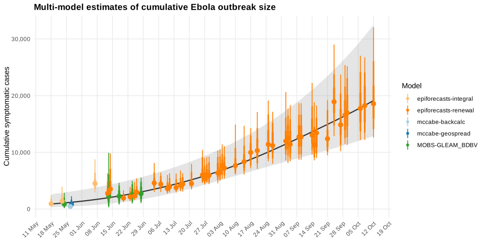
Multi-model estimates of cumulative Ebola outbreak size
Each colored point interval shows an individual model’s median (point) with 50%, 80%, and 95% uncertainty intervals. The grey band and line show a smoothed quantile-averaging ensemble (GAM spline fit to the 2.5th, 50th, and 97.5th percentiles across all models on a log10 scale).
Data: BDBV Modeling Hub model-output submissions, dated 18 May 2026–12 Oct 2026.
Source: github
Synthesizing evidence
State of the evidence
The body of evidence comprises ten analyses, including peer-reviewed studies, preprints and two online dashboards, posted from 24 May to 10 October 2026. Only McCabe et al., Abbott et al., Epistorm, Oraby et al. and Kim et al. estimate true outbreak size or an upper bound of it. Mooring et al. and Chamla et al. project future trajectories, while the three Verheyden preprints address growth, fatality ratios or forecasting of confirmed counts to give wider context on the question of outbreak size.
How the estimates compare
Abbott et al. estimate roughly 1.6–3.3× as many infections as laboratory-confirmed cases at 10 October.[1][2][3] McCabe et al. estimated about 280–2,520 cases at 27 May, against 1,031 suspected-or-confirmed reported cases, so the range spans values below and above the reported figure.[4][5] Chamla et al. report that the suspected count peaked at 1,077 on 26 May and was then sharply revised downward, so the laboratory-confirmed series became the reliable comparator;[6] a suspected-or-confirmed denominator such as McCabe et al.'s is therefore not equivalent to a confirmed count. Oraby et al. estimate 1,120 cumulative infections at the fitted rate at which patients leave isolation against 896 confirmed cases as of 17 June, without stating a ratio.[7][8] The analyses differ in denominator, geography and method, and the denominator alone matters: Chamla et al.'s published quantity is the confirmed-case count, which excludes the unconfirmed and unascertained cases that Abbott et al. and McCabe et al. estimate.[9]
Key uncertainties and assumptions
Most of the uncertainty is structural rather than statistical, and four assumptions are shared widely enough that their failure would move several estimates together.
First, the analyses make different assumptions about detection, so their estimates are not measuring quite the same thing. Chamla et al. set the reporting fraction at 1.0, which limits their quantity to confirmed cases;[10][9] Epistorm’s second calibration stage allows ascertainment as low as 40%;[11] and Abbott et al. have no line list or reporting-completeness data to anchor detection, so their multiplier of roughly 1.6–3.3 infections per confirmed case is a model-based extrapolation.[12][2]
Second, death-based estimates rest on borrowed parameters. McCabe et al. assume a case fatality ratio and onset-to-death delay consistent with earlier Bundibugyo outbreaks and an assumed epidemic doubling time of 7–14 days (a 10-day doubling time in the main scenario), and the estimated size rises with a lower ratio, faster growth, or a higher share of deaths due to Ebola.[13][14][15] Abbott et al. likewise use weakly informed priors for delays and the ratio, often from other outbreaks, and their posteriors largely track those priors.[16]
Third, travel-based inference assumes every resident is equally likely to travel regardless of infection status, which healthcare-seeking behaviour violates.[17] Short trips also let infected travellers return home before detection, and accounting for trip durations raised Kim et al.'s central estimates and widened their confidence intervals.[18][19]
Finally, model simplifications limit what the estimates can show. Chamla et al. assume homogeneous mixing and uniform response intensity, which oversimplify spatial heterogeneity across health zones, and anchoring on a single confirmed-case datum makes their fit sensitive to that anchor.[20] Oraby et al. add that the undetected burden, postmortem detection and funeral infectiousness cannot be separately identified, so several parameters were fixed or strongly regularized.[21]
What would reduce uncertainty
Chamla et al. and Verheyden and Mudogo both name line-list data as a priority, with Chamla et al. adding contact-tracing data.[22][23] Additionally, in line with their shared uncertainties, would be outbreak-specific cross-border movement data, because travel-based methods are limited by poorly understood crossing dynamics[24] and the export stream in Abbott et al. rests on a traveller volume taken from McCabe et al.[25][26]
Open questions
The authors’ open questions converge on better linked data. McCabe et al. call for epidemic size, growth rate, and geography to be characterised with epidemiological and genomic data, while Chamla et al. call for line lists, contact-tracing data, and dynamic mobility estimates.[27][22] Verheyden and Mudogo identify patient-linked records as necessary for causal attribution of fatality differences.[28]
What this means for the response
The evidence suggests confirmed counts should be treated as a lower bound, rather than as the true number of cases as the underascertainment rate remains modest-to-substantial.[2][29][7]
Individual analyses
Abbott et al. (10 Oct 2026)
Estimating the current size of the 2026 DRC Bundibugyo virus outbreak
Overview
This analysis estimates how many people have been infected in the DRC outbreak, reported and unreported, and how that compares with laboratory-confirmed cases. It fits a single statistical model of how infections spread to several streams of situation-report counts and to cases exported to Uganda. The outbreak is estimated to have caused 30% 18406-21567, 60% 16546-23965, 90% 14028-29258 infections to date, reported and unreported.[1] Against the 8978 laboratory-confirmed cases by the cut-off, that is roughly 1.6-3.3× as many infections.[2]
Estimate
Headline (joint model, DRC nationally, data as of 10 October 2026): Cumulative infections, reported and unreported, are estimated at 30% 18406-21567, 60% 16546-23965, 90% 14028-29258.[1] Against the 8978 laboratory-confirmed cases by the cut-off, this is roughly 1.6-3.3× as many infections, so confirmed cases are estimated to capture only a small share of the outbreak.[2]
Other quantities reported at the same cut-off:
The outbreak is estimated to have begun between 2026-03-01 and 2026-03-27 (90% interval), an elapsed age of 197-223 days.[30]
The initial reproduction number was 30% 1.91-2.18, 60% 1.79-2.38, 90% 1.59-2.73, and the latest is 30% 1.05-1.2, 60% 0.97-1.3, 90% 0.83-1.52.[31]
The latest growth rate is 30% 0.003-0.014, 60% -0.002-0.021, 90% -0.013-0.035 per day.[32]
The case-fatality ratio is 30% 0.46-0.51, 60% 0.43-0.54, 90% 0.39-0.6.[33]
The page does not give numeric infection estimates for the earlier frozen cut-offs or the per-stream fits in the text provided.
Methods
Joint Bayesian multi-patch renewal model: This is a real-time, joint Bayesian model that began as a replication of McCabe and others (2026)[34]. One joint model is fitted to every national data stream and the provincial tables, on a daily grid from a seeding date to the cut-off.[35] Each patch runs its own renewal equation, with a reproduction number that is a shared weekly trend times a deviation for that patch.[36] Each data stream sees a delayed or thinned view of the same patch infections.[37] The streams include suspected and confirmed cases and deaths, laboratory volumes, treatment-centre flows, a digitised symptom-onset curve and Uganda exports. Outbreak size and each system’s reporting fraction are estimated jointly.[38] It covers the DRC nationally by province, with Uganda exports as an additional data stream. Importation couples the patches by moving a share of each day’s new infections from one patch to another.[39] The outbreak is assumed to have started from a zoonotic spillover and to have grown through an unobserved cryptic exponential phase.[40] A genetic bound bounds the cryptic phase from below.[41]
Health-zone model: A second model splits the joint model’s infections in each patch across the health zones of that patch. It is fitted after the joint model, to the same cut-off, and does not feed back into it.[42] It uses the cumulative confirmed cases and deaths for each health zone from the situation reports. It produces zone-level reproduction numbers and one-week forecasts.
Single-stream fits, frozen re-fits and forecasts: Single-stream models are written for each count-based stream, so each stream’s posterior outbreak size can be compared with the joint.[43] Frozen re-fits cut the data to an earlier cut-off and re-fit the joint model.[44] Forecasts are drawn from the fitted model itself.[45]
Assumptions
Generation interval and seeding: The generation interval is a Gamma with a sampled mean and SD, taken from the Ebola virus disease serial interval used as a generation-time proxy (mean 15.3 d, SD 9.3 d).[46] The outbreak is assumed to have started from a zoonotic spillover and grown deterministically through an unobserved cryptic exponential phase.[40] The origin prior is centred so the implied origin sits in mid-February, with 90% of its mass between mid-January and mid-March.[47] The initial growth rate has a log-normal prior equivalent to a doubling time centred on 11.7 d.[48] The authors state the model inherits McCabe et al.'s assumptions of a single zoonotic seed and a generation interval from earlier Ebola outbreaks, which help constrain the estimated outbreak age and early reproduction number.[49]
Genetic bound on outbreak age: The TMRCA is treated as a lower bound on the outbreak age, leaving the age free above it.[50][51] The molecular clock is fixed to the rate of the 2013-2016 West African Ebola epidemic.[52] The authors state they fix the clock and do not propagate cross-outbreak or clock uncertainty.[53]
Response effect on transmission: The response is assumed to take about three weeks (21 days) to take effect and to be able only to reduce transmission.[54] The ramp is fixed in time, with an assumed start and three-week duration, and only its size is estimated.[55]
Incubation and other delays: Incubation uses the 2007 Uganda outbreak estimate (mean 6.3 d).[56] Onset-to-admission is a Gamma centred on the Isiro reanalysis posterior (implied mean about 4 d).[57] Onset-to-death is the convolution of onset-to-admission and admission-to-death (implied mean about 13 d).[58] The authors state that nearly all of the delays rest on weakly-informed priors, often from other outbreaks, and that their posteriors largely track those priors.[16] The onset-to-report delay is the exception, informed by the onset curve.[59]
Case-fatality ratio: The prior is Beta(6.6, 13.4)[60], with a mean that matches the CDC figure and the corrected central CFR in the 20 May report (McCabe and others, 2026).[61] The authors say the CFR prior’s posterior largely tracks the prior.[16]
Ascertainment and non-BVD background: Two surveillance systems, DRC passive community surveillance and Uganda point-of-entry/hospital surveillance, each capture a fraction of the true cases passing through them.[62] The prior reflects the active case-finding of a declared Ebola response.[63] The code centres the prior at logit(0.75)[64]. Reported suspected cases include an additive non-BVD background.[65] The background is inferred to be the majority of the suspect pool.[66] The DRC ascertainment, testing fraction and specimens analysed per suspect are each one value over the window, although ascertainment probably rose, so a change in any of them is read as a change in incidence.[67]
Laboratory assumptions: Confirmation runs on the altona RealStar Filovirus Screen RT-PCR.[68] The effective process sensitivity is about 98% with two controls, so the sensitivity prior is centred there.[69] The severity-enrichment priors are not set from data.[70]
Cross-border travel: The source population is fixed, and the traveller volume is given a Normal prior around the McCabe et al. figure.[26] The export model counts every border crossing by an undetected infection as a possible detection in Uganda. A constant share of round trips is absorbed into the Uganda ascertainment, but a share that changes over the window is not.[71]
Spatial structure and stream independence: The streams observe overlapping people but are fitted as conditionally independent given latent incidence, which can understate uncertainty.[72] Ituri, Nord-Kivu and Haut-Uele are modelled individually, every other affected province is pooled into a fourth patch, and each is well mixed.[73] The gravity kernel coupling the provinces is assumed, not measured, as there is no mobility or origin-destination data.[74]
Limitations
Aggregate data and model-based extrapolation: The authors do not have a line list, information on case definitions or reporting completeness, or access to the response’s internal data. Every estimate is therefore a model-based extrapolation under strong assumptions, not a measurement.[12] The work is done outside the outbreak response, so changes in reporting practice are inferred from the reports rather than known.[75] Almost every count is report-dated, so the epidemic’s timing is recovered mainly through the assumed delays.[76]
Status of the analysis: The code and analysis were drafted by a language model and reviewed by people and by language models.[77] The report is re-run as new data arrive, so the estimates change between updates, and it has not been peer reviewed.[78]
Borrowed priors: Most quantities, including nearly all of the delays, the CFR and the laboratory assumptions, rest on weakly-informed priors, often from other outbreaks, and their posteriors largely track those priors.[16] The onset-to-death delay and the genetic seeding bound do not propagate cross-outbreak or clock uncertainty.[79]
Data revisions and discontinued streams: Later situation reports can revise earlier totals up or down as suspects are reclassified and newly-reporting health zones are added, and this revision process is not modelled.[80] The suspected streams are no longer published, so the late window rests on the confirmed, laboratory, treatment-centre and onset data, and the suspected forecasts cannot be checked.[81] The onset curve is digitised from a figure that each report redraws, so the counts carry scan error that the model treats as noise at a fixed scale.[82]
Stream independence: The streams are fitted as conditionally independent given latent incidence, which can understate uncertainty.[72]
Spatial and bed-model simplifications: The treatment-centre model carries one national bed capacity and demand, so it cannot represent local saturation. Ituri holds most of the occupied beds, so the national bed shortfall understates local unmet need.[83] Spread inside a province is not represented.[73] The province tables start on 15 June, and before then the provinces are informed only through the national streams.[84] The zone stage is melded one way onto the joint fit, so the zone data do not update or correct the national and province estimates.[85]
Sampling diagnostics: The joint fit passes the convergence checks with warnings.[86] Its worst R-hat is 1.04 and its lowest bulk effective sample size is 43.[87] Across all 12 fits the worst R-hat is 1.19, and the lowest bulk effective sample size is 13, both in the deaths (DRC) fit.[88]
Data sources
Primary outbreak data:
DRC situation reports: the DRC data come from the situation reports of the Institut National de Santé Publique (INSP, 2026).[89]
Confirmed totals: 8978 confirmed cases and 4336 confirmed deaths at 2026-10-10.[90]
Suspected totals, frozen after reclassification: 246 suspected deaths and 1077 suspected cases at 2026-05-26.[91]
Daily new-suspect counts: read from 4 June[92].
Laboratory data: 755 specimens analysed at 2026-05-28.[93]
Digitised onset curve: from SitRep 059 (12 July) onward, a raster figure of confirmed cases by symptom-onset date, digitised directly from the figure.[94] The last total is 7132 at 2026-10-10.[95]
Treatment-centre data: a patient-movement table (Tableau 6) from 13 June.[96] At 2026-08-02 it shows 147 admissions, 22 in-care deaths, 93 rule-outs and 2 absconded.[97]
Provincial and zone tables: Tableau 2 of the same situation reports.[98]
Uganda exports: the cases and the one death exported across the border, from WHO situation reports and Disease Outbreak News.[99] Three exported cases were dated 2026-05-23 and one export death 2026-05-14.[100]
Auxiliary data:
Travel and population: cross-border traveller volume and source population from McCabe and others (2026).[25] The traveller prior mean is 1871 (SD 200), and the source population is 4392200.[101]
Province and zone geography: 2019 province populations from the DRC’s Institut National de la Statistique.[102] Distances use WorldPop-weighted population centres.[103]
Genetic data: a BEAST time tree of the first ten sequenced genomes places the TMRCA at a mean of 25 March 2026.[104] A BEAST X reanalysis of 139 BDBV genomes reports an exponential-growth doubling time of 11.7 d (95% HPD 6.8-17.5).[105]
Generation interval: Ebola virus disease serial interval (fitted Gamma, mean 15.3 d, SD 9.3 d, from 92 transmission pairs; WHO Ebola Response Team 2014).[106]
Incubation period: from the 2007 Uganda outbreak (mean 6.3 d, 95% CI 5.2-7.3; MacNeil et al., 2010).[56]
Onset-to-admission and onset-to-death delays: a Bayesian reanalysis (Funk and Abbott, 2026) of the 2012 Isiro Bundibugyo virus outbreak line list (Rosello and others, 2015).[107]
Case-fatality prior: the CDC summary for the two previous BVD outbreaks.[108]
Verheyden and Mudogo (13 Sep 2026)
Observed Fatality or Observed Death? Differential Death Ascertainment and Provincial Mortality Heterogeneity during the 2026 Bundibugyo Virus Disease Epidemic in the Democratic Republic of the Congo
Overview
This analysis does not attempt to estimate the true size of the 2026 BVD outbreak or a detection multiplier for total infections. Instead, it investigates why North Kivu reported a substantially higher cumulative case-fatality ratio (CFR) than Ituri Province, using a longitudinal reconstruction of DRC national situation reports (SitReps) through 13 September 2026. The central finding is that 415/1,507 (27.5%) classified positives in Ituri and 265/568 (46.7%) in North Kivu were already deceased when reported positive (Mantel-Haenszel OR 2.18, 95% CI 1.76-2.70)[109], indicating that differential ascertainment (detection of cases alive versus after death) is a major driver of the provincial CFR gap rather than necessarily reflecting a true outbreak-size discrepancy.
Estimate
The analysis does not produce an estimate of true outbreak size or a detection multiplier relative to confirmed cases. It reports only reported/confirmed case and death counts and CFR-related quantities. For context, confirmed cumulative counts at the freeze were by 13 September, the formal freeze, Ituri reported 5,659 cases and 2,583 deaths (45.6%) and North Kivu 1,281 cases and 797 deaths (62.2%), a 16.6-point gap[110]. The key quantitative outputs are the dead-at-detection proportions (27.5% Ituri vs 46.7% North Kivu, Mantel-Haenszel OR 2.18, 95% CI 1.76–2.70) and the counterfactual compatibility calculation showing that applying a common 25% fatality rate among live-detected cases to the late-regime dead-at-detection shares would generate expected reported CFRs of 45.7% and 61.5%, respectively[111], close to the observed 13 September CFRs. No estimate of true infection numbers or under-ascertainment multiplier for total case burden is given.
Methods
Longitudinal ecological surveillance reconstruction: The authors designed a longitudinal ecological surveillance analysis using official DRC Institut National de Santé Publique (INSP) situation reports from the 17th Ebola epidemic[112], organized at province-by-SitRep level, to compare the proportion of newly confirmed cases already dead when detected (“dead-at-detection share”) between Ituri and North Kivu provinces.
Matched-SitRep comparison with Mantel-Haenszel and Bayesian binomial logistic modeling: The core analysis restricted comparisons to SitReps in which both Ituri and North Kivu contain definitionally compatible living/deceased splits[113], then used a Mantel-Haenszel comparison stratified by SitRep[114] alongside a Bayesian binomial logistic model...fitted as a complementary analysis with province, reporting regime, and their interaction[115], applied to the same two-province dataset of 28 matched SitReps.
Counterfactual standardization (compatibility calculation): This method used a simple accounting identity, If π is the proportion of confirmed cases already deceased when detected and q is the eventual fatality among cases detected alive, then under a two-pathway completed-outcome accounting model the expected reported CFR is R = π + q(1-π)[116], applied to the same Ituri/North Kivu provincial data to test whether ascertainment differences alone could reproduce the observed CFR gap, varying q from 0.10 to 0.50.
Postmortem-surveillance and death-location triangulation: Using operational indicators such as bodies swabbed relative to death alerts and death-location classification (community, health facility, CTE/CT), the analysis triangulated independent evidence of differential postmortem detection between the two provinces, e.g. in the three matched SitReps for which a comparable death-alert denominator and number of bodies swabbed could be reconstructed (72, 80 and 82), Ituri reported 163 bodies swabbed for 247 death alerts (66.0%), whereas North Kivu reported 118 for 120 (98.3%)[117].
None of these methods estimate a true outbreak size or a detection multiplier for total infections; the analysis is explicit that it does not attempt latent incidence estimation: We did not fit a more elaborate latent epidemic simulation because the aggregate SitRep streams do not independently identify true incidence, outcome-specific detection probabilities, and biological fatality.[118]
Assumptions
Two-pathway accounting structure: The counterfactual calculation assumes cases enter the confirmed series via only two pathways — detected alive or detected after death — formalized as If π is the proportion of confirmed cases already deceased when detected and q is the eventual fatality among cases detected alive, then under a two-pathway completed-outcome accounting model the expected reported CFR is R = π + q(1-π)[116]. The authors are explicit this is a compatibility analysis, not an estimator of infection-fatality risk[119].
Common eventual fatality (q) across provinces: The compatibility calculation assumes a shared eventual fatality probability among live-detected cases, tested across q values from 0.10 to 0.50[120], with an illustrative common value of 25% used to reproduce observed CFRs. This is explicitly a sensitivity sweep rather than a fixed single value.
Non-identifiability of latent incidence and fatality: The analysis structurally assumes it cannot and should not attempt to decompose true incidence, biological fatality, and ascertainment from aggregate counts alone, stating with aggregate SitRep counts alone, true incidence, biological fatality, live-case detection, and postmortem detection are not separately identifiable without strong external constraints[121], and treating this as a deliberate stop rule: when materially different combinations of latent incidence, fatality, and ascertainment can generate the same observed streams, the data do not support a unique decomposition[122].
Stratification by reporting regime rather than a constant province effect: Because the report-specific odds were heterogeneous, we did not interpret one common odds ratio as a time-invariant biological effect[123], the analysis assumes the ascertainment contrast varies by reporting regime (COUSP period SitReps 66-77 vs Task Force period 96-122) rather than being constant over time, and models this with a Bayesian province-by-regime interaction using weakly informative priors Weakly informative Normal(0, 2.5) priors were used for contrast coefficients and a wider Normal(0, 5) prior for the intercept[124].
Missingness treated as non-random and non-imputed: The analysis assumes missing fields should not be filled in, stating Missingness was treated as a feature of the surveillance record. We did not impute zero for absent fields and did not interpolate the primary living/deceased split across reports.[125]
Limitations
Aggregate, unlinked data: The authors state that the SitReps are aggregate operational reports rather than linked patient-level datasets, so a death classified in the laboratory section cannot be linked to an alert, admission, treatment history, symptom-onset date, or individual outcome trajectory.[126]
Changing definitions and reconciliation: The authors note reporting definitions changed over time, some reports contain reconciliation corrections, and several operational fields are absent or incomplete.[127] Relatedly, the primary split is available only on selected reports and may itself reflect which samples reached the laboratory.[128]
Non-identifiability of biological fatality: The authors emphasize that neither the matched analysis nor the counterfactual standardization identifies the true infection-fatality risk. A latent decomposition would require patient-linked data or strong external constraints; without them, multiple combinations of incidence, mortality, and ascertainment remain observationally compatible.[129]
Operational indicators not patient-linked: Postmortem swabbing and death-alert counts used for triangulation are described as limited: these are aggregate operational completion indicators; alert and swab counts are not patient-linked and can include carry-over.[130]
Cannot rule out genuine clinical/capacity differences: The authors acknowledge the source-audited and model-based analyses support an ascertainment mechanism but also leave a credible pathway through which delayed presentation and constrained care could contribute to genuine mortality differences.[131]
Health-zone analysis limited: Health-zone data confirm that neither province is internally homogeneous, but the current SitRep series does not provide the primary living/deceased laboratory split consistently at health-zone level.[132]
Cannot quantify effect of parallel administrative structure: Regarding the AFC/M23-administered response in parts of North Kivu, the authors state we cannot quantify this pathway from the available aggregate SitReps, and offer it as one plausible, non-mutually-exclusive mechanism rather than an identified cause.[133]
Data sources
Primary outbreak data: the analysis relies on official DRC Institut National de Santé Publique (INSP) situation reports from the 17th Ebola epidemic[112], with twenty-eight SitReps provid[ing] a matched provincial living/deceased laboratory split[134] forming the primary inferential series (SitReps 66, 67, 69, 70, 72, 73, 74, 77, 96, 97, 99, 101, 102, 104, 105, 108, 109, 110, 111, 112, 113, 114, 115, 116, 117, 118, 119 and 122, per the document). Across these, the laboratory stream classified 1,507 new/report-period positives in Ituri, of whom 415 were deceased (27.5%), and 568 in North Kivu, of whom 265 were deceased (46.7%)[135]. Additional primary streams include provincial cumulative confirmed case/death counts, death-location classifications (community/health facility/CTE), postmortem swabbing and death-alert cascades, and hospital bed-occupancy data, all drawn from the same SitRep sequence.
Auxiliary data: the analysis references prior literature on ascertainment bias in outbreak fatality estimates and historical operational context, e.g. postmortem Ebola testing was operationalized in eastern DRC during and after the 2018-2020 epidemic, while community-based surveillance systems expanded the production and investigation of alerts and improved access to testing[136], and notes on a contemporary patient-level analysis from the same outbreak Contemporary patient-level reporting from the same outbreak has already cautioned that early observed deaths cannot be interpreted as a CFR when final outcomes and denominators are incomplete[137]. No travel, demographic, or cross-border datasets are used, as the analysis is confined to within-DRC provincial surveillance comparison.
Epistorm (27 Jul 2026)
Ebola Bundibugyo Virus — DRC · Spread Risk Assessment #7 · Local Transmission Scenarios
Overview
This analysis uses a stochastic, metapopulation transmission model (built on the GLEAM framework) to project the trajectory of the DRC Bundibugyo virus disease outbreak under different isolation-intervention scenarios, rather than to produce a single “true size” nowcast. The report presents a stochastic, metapopulation transmission model built using the GLEAM framework, incorporating transmission occurring in the hospital, community, and through funerals, and explicitly modeling isolation protocols through ETC.[138] The model is calibrated against confirmed Ituri case counts allowing for under-ascertainment, yielding posterior R₀ ≈ 2.02 (90% CrI [1.72, 2.47]) and empirical doubling time 12.9 d (90% CrI [10.7, 15.6])[139], and forward projections across three isolation scenarios (30%, 50%, 75%) show widely diverging outcomes by 30 September 2026, ranging from near-control under high isolation to outbreak sizes exceeding 20,000 cases in three-quarters of trajectories under low isolation.
Estimate
The calibration itself implies a range for true cumulative symptomatic cases in Ituri as of 18 July 2026: the simulated cumulative symptomatic onsets in Ituri by 18 July are required to lie in the window [2,090, 5,225], allowing ascertainment as low as 40%[11], against a confirmed count of 2,090 at that date.
For forward projection to 1 August 2026 (DRC-wide), the headline figures are: Cumulative symptomatic cases: iso30 5,551 [3,352 - 8,245], iso50 4,991 [2,981 - 7,318], iso75 4,414 [2,645 - 6,363][140], with active cases (I + H + ETC): iso30 1,287 [651 - 2,342], iso50 870 [423 - 1,630], iso75 462 [206 - 946][141] and new symptomatic cases per day: iso30 158 [75 - 298], iso50 95 [44 - 195], iso75 42 [16 - 96][142].
For 30 September 2026, outcomes are reported as probabilities rather than point estimates: probability of ≥20,000 cumulative symptomatic cases is <1% under 75% isolation, 20% under 50%, and 75% under 30%[143]; and the probability of exceeding 10,000 cases by 30 September is 98% under 30% isolation, 69% under 50% and 9% under 75%, while for the higher threshold of ≥20,000 cases the corresponding probabilities are 75%, 20% and <1%[144].
Methods
GLEAM metapopulation model with care-pathway SEIHFR dynamics: This is a stochastic, spatially explicit simulation model in which GLEAM (Global Epidemic and Mobility Model) is an Africa-wide metapopulation network coupled by daily commuting matrices and origin-destination passenger flows, with within-basin compartmental dynamics simulated as a discrete-time multinomial chain-binomial process[145]. The compartmental structure follows a Legrand-like SEIHFR scheme, extended to incorporate three potential outcomes an infectious individual could experience[146] — community, HCF-only, and isolation-to-ETC branches — and it applies to DRC (17 basins plus Goma) and Uganda.
Two-stage Approximate Bayesian Computation calibration: The model’s epidemiological parameters are fitted to outbreak data using ABC rather than a direct estimator. Stage 1 conditions on observed cross-border importations from Ituri to Uganda, requiring exactly one Uganda importation by 14 May 2026 and exactly one further importation in the window 14 to 18 May 2026.[147] Stage 2 conditions the Stage-1 posterior on the cumulative laboratory-confirmed count in Ituri at 18 July 2026 (2,090 cases) allowing ascertainment as low as 40%, requiring the simulated cumulative symptomatic onsets in Ituri by 18 July to lie in the window [2,090, 5,225].[11] This calibration applies to the Ituri source population within DRC, with sensitivity noted in that posterior medians of R₀ and Td are stable when the ascertainment floor is relaxed or tightened, though a formal sensitivity table at alternative floors is deferred to a subsequent update[148].
Scenario-based forward projection: Using the calibrated posterior, the model projects DRC-wide outcomes under three isolation targets. Forward projections evaluate three target isolation rates, 30%, 50% and 75%, each phased in at 2 percentage points per day from 20 May 2026 across DRC (17 basins plus the Goma catchment) until the scenario target is reached, while Uganda is held at a constant 80% isolation from the start of the intervention window.[149] This produces cumulative case, active case, daily incidence, and Rt trajectories, plus probabilities of exceeding case thresholds, all aggregated to DRC.
Assumptions
Calibration priors: The model draws R₀ from U(1.2, 5.0), incubation period TE from U(5, 10) days (Erlang-2, two-stage latent), and outbreak start date from U(15 Feb, 15 Mar 2026)[150], with these priors filtered through the two-stage ABC against importation and case-count evidence.
Ascertainment floor: The baseline analysis allows ascertainment as low as 40% (window [2,090, 5,225])[151] when calibrating to the 18 July Ituri confirmed count; this single assumption directly sets the implied detection gap used to anchor the model.
Care-pathway dwell times and case-fatality ratios: The model fixes compartment-specific parameters including community dwell time 9.6 d, onset-to-HCF 5 d (routine) vs 2 d (isolation track), HCF-to-ETC transit 3 d, HCF stay 4.6 d, funeral period 2 d, HCF admission probability 0.80, CFR of 0.50 (non-hospitalised), 0.45 (regular HCF), 0.30 (ETC), an R₀ split of 0.44:0.22:0.34 across community/HCF/funeral transmission, and a residual HCF-isolation transmission factor of 0.1[152], several sourced from literature/prior outbreaks.
Isolation ramp and intervention structure: Isolation is phased in at 2 percentage points per day from 20 May 2026 across DRC (17 basins plus Goma) until reaching target (30%, 50%, or 75%), with Uganda held at a constant 80% isolation[149], and this ramp and case-finding timing are applied homogeneously across all symptomatic cases, though real-world coverage varies by location and over time[153].
Mobility and seeding: No mobility reductions between subpopulations are assumed — no behavioral reduction, no border closure, and no seasonality in transmissibility is modeled[154][155], and the epidemic is seeded with 5 infectious cases in Ituri on the inferred start date, with every other basin fully susceptible and reached only through mobility[156].
Limitations
Calibration data is limited to a single date and sparse importation counts: Stage 1 uses only evidence of importations from Ituri → Uganda (exact-count, no tolerance band), without directly fitting within-Ituri incidence, while Stage 2 adds only a single cumulative count at one date.[157] Alternative acceptance rules or additional within-basin time-points would shift the posteriors.[158]
Projections beyond the calibration date are model-driven: Calibration extends only to the 18 July 2026 confirmed-case evidence, and projections beyond that date are model-driven and depend on assumptions about isolation timing and intensity.[159]
Borrowed timing parameters may not match 2026 operations: Isolation-track timings (Tiso = 2 d, HCF → ETC ≈ 3 d) follow the 2018 North Kivu RVEAP response, which may not exactly match the 2026 operational reality.[160] The residual nosocomial channel in the iso branch (0.1·βH) is a modelling assumption, sensitivity-testable.[161]
Static mobility and homogeneous intervention coverage: Mobility is held static across the simulation, with no behavioral reduction, no border closure modeled, and no seasonality in transmissibility; informal cross-border movement may be under-captured.[162] The isolation ramp and case-finding timings are applied homogeneously across all symptomatic cases, while real-world coverage varies by location and over time.[153]
Scope exclusion: International dissemination is out of scope for this report (see Reports #3 and #4).[163]
Data sources
Primary outbreak data: DRC cumulative laboratory-confirmed cases (3,360) and confirmed deaths (1,487) as of 27 July 2026 across 48 health zones in five provinces, with 733 patients currently hospitalised in isolation[164]; Uganda confirmed cases (20, including 2 deaths)[165]; the Ituri confirmed case count used for calibration, 2,090 cases as of 18 July 2026[166]; and cross-border importation event counts used in Stage 1 calibration, requiring exactly one Uganda importation by 14 May 2026 and exactly one further importation in the window 14 to 18 May 2026[167].
Auxiliary data: IATA / OAG passenger origin-destination data and daily commuting matrices for mobility coupling[168][169]; natural-history parameters from the 2007-2008 Uganda BVD outbreak data (Wamala et al.)[170]; and case-finding timing parameters following the 2018 North Kivu RVEAP response[171].
Verheyden and Mudogo (27 Jul 2026)
Sixteen Days Undetected: Growth Dynamics and the Case for Pre-Positioned Response Capacity in the 2026 Bundibugyo Virus Disease
Outbreak, Democratic Republic of the Congo
Overview
This analysis aims to characterize, rather than estimate a single “true size” figure for, the 2026 BDBV outbreak: specifically its early growth rate, the date transmission actually began (back-calculated), and whether the rising case-fatality ratio reflects worsening severity or a detection artefact. The authors analysed a corrected daily surveillance series (65 observations, 14 May-27 July 2026) using non-linear least-squares regression and a Bayesian Poisson growth model fitted by Markov chain Monte Carlo, with five sensitivity analyses.[172] The headline findings are that early confirmed cases grew at 0·1261 per day (95% CI 0·0885-0·1636), a doubling time of 5·50 days (4·24-7·83), three-fold faster than previous BDBV outbreaks (15-18 days); Bayesian back-calculation placed transmission onset on 19 April 2026 (95% highest-density interval 9-27 April), 16 days before the WHO alert and 25 days before laboratory confirmation; and confirmed case-fatality ratio rose from 12·1% to 44·3%, with a cross-classification analysis supporting progressive reclassification rather than increasing virulence.[173] A later full-series logistic model produces a provisional outbreak-size (final-size, K) projection, but the authors flag this estimate as unstable across successive data extensions.
Estimate
This analysis does not produce a single “true outbreak size” figure comparable to under-ascertainment models; its primary quantitative outputs are growth rate, doubling time, and back-calculated onset date. Two quantities come closest to a case-burden estimate. First, back-calculated circulating-case numbers at key pre-declaration dates: at a doubling time of 5·5 days, this detection lag alone corresponds to approximately six-fold case growth before international response mechanisms activated: at the WHO alert date, the model implies 4-13 circulating cases (median 8); by declaration on 15 May, 20-38 cases (median 28).[174] Second, a provisional final-size (K) projection from the full-series logistic model: over the full 65-observation series (14 May-27 July), growth rate fell to r = 0·0364 per day (Tᵈ = 19·02 days), and a logistic model was preferred by AIC (K ≈ 6,166), confirming substantial deceleration as response capacity scaled - though the authors treat this plateau estimate as provisional: successive one-week extensions of this series have shifted the fitted asymptote from K ≈ 2,333 to K ≈ 3,002 to K ≈ 6,166 (29% then 105% change).[175] The most recent logistic K estimate carries a 95% CI of 4413-7920.[176] The authors explicitly caution that this figure has more than doubled across two successive one-week extensions of the data window and is reported here for model-comparison completeness, not as a dependable final-size projection.[177]
Methods
Classical growth-rate regression: Cumulative case counts C(t) were modelled as C(t) = C₀·exp(r·t), where r is the exponential growth rate and doubling time Tᵈ = ln(2)/r; the early-phase model (14-27 May, pre-discontinuity) was fitted by non-linear least squares to 12 daily observations, and a logistic model was fitted to the full 65-observation series and compared against the exponential model by Akaike Information Criterion.[178] This method is applied to DRC-national confirmed daily case counts.
Bayesian hierarchical growth/back-calculation model: A Bayesian hierarchical model (Poisson likelihood, weakly informative Normal priors, fitted by Markov Chain Monte Carlo in PyMC3) estimated growth rate r, initial case count C₀, and t_back - the number of days before the first situation report that transmission began - with full posterior uncertainty propagation.[179] (The verified implementation used a Normal rather than Poisson likelihood with an estimated observation-noise scale.) It is applied to the same DRC-national pre-discontinuity daily series, with five pre-specified sensitivity analyses varying priors, the fitting window, and the observation-model distribution.
CFR trajectory and cross-classification analysis: CFR was calculated at each reporting date; at the earliest date with disaggregated confirmed and suspected case and death data (21 May 2026), confirmed and suspected CFR were compared by two-sample z-test, and the temporal CFR trajectory was examined for consistency with progressive reclassification of suspected deaths into the confirmed category versus an irregular pattern consistent with genuine severity change.[180] This uses DRC-national aggregate surveillance data, supplemented by a single cross-classification snapshot from external sources.
Assumptions
Growth-model functional form: Cumulative case counts were modelled as C(t) = C₀·exp(r·t)[181] for the early phase, with a logistic alternative, C(t) = K / [1 + ((K − C₀)/C₀)·exp(−r·t)],[182] fitted to the full series. The choice between exponential and logistic forms drives the instability in the final-size (K) estimate.
Bayesian priors: Weakly informative priors were used: r ∼ Normal(0.13, 0.05), C₀ ∼ Normal(33, 10), σ ∼ HalfNormal(20).[183] Sensitivity analyses varied these: an optimistic prior (r ∼ Normal(0.11, 0.02)) gave posterior median r = 0.124 and implied onset 17 April, while a pessimistic prior (r ∼ Normal(0.15, 0.03)) gave posterior median r = 0.137 and implied onset 20 April,[184] with back-calculated onset across these variants ranging 17-22 April consistent with the primary estimate (19 April, 95% HDI 9-27 April).[185]
Single index case: The back-calculated parameter t_back gives the outbreak start date assuming a single index case (C = 1) at the back-calculated start.[186] Back-calculation assumes a single index case; multiple early spillover events (as suggested for the 2012 BDBV outbreak) would shift the estimated start date later, making 19 April a conservative (earlier) estimate under the single-introduction assumption.[187]
Mongbwalu cluster excluded from formal estimation: The authors do not incorporate reported evidence of a possible earlier, undetected February 2026 death cluster into the formal back-calculation, which would launder soft, uncertain evidence into false statistical precision, and instead report it as an explicit plausibility bound: if this cluster reflects genuine early BDBV transmission, true onset could lie anywhere between early February 2026 and the estimate of 19 April 2026.[188]
Limitations
Historical comparison data are approximate: Historical BDBV doubling-time comparisons are approximate; formal statistical comparison requires digitised onset curves from 2007 and 2012 primary sources, which are ongoing.[189]
Single index case assumption: Back-calculation assumes a single index case; multiple early spillover events would shift the estimated start date later, making 19 April a conservative (earlier) estimate under the single-introduction assumption.[187]
CFR interpretation based on limited data: CFR interpretation rests on aggregate surveillance data and a single cross-classification snapshot; line-list data stratified by onset date, confirmation date, care setting, and outcome would enable formal survival analysis.[23]
Mechanistic explanations are inferential: The mechanistic discussion of growth-rate drivers is inferential; testing any individual mechanism requires appropriately controlled epidemiological studies.[190]
Final-size projection is unstable: The epidemic curve does not yet contain enough information to fix a final size with confidence - a caveat substantiated directly where extending the data window by a further week nearly doubled the logistic model’s estimated final size.[191]
Data completeness and corrections: The daily series is not entirely complete: ten dates lack confirmed-case counts in the primary source and were excluded rather than interpolated - a larger set than an earlier draft of this manuscript reported (five dates), which is flagged for the authors to reconcile rather than silently revised.[192] Earlier weekly-aggregated extractions were superseded: the original analysis relied on weekly aggregated case counts (n = 3 for the early-phase model); this has been resolved using the complete corrected daily surveillance series.[193]
Uncorroborated earlier cluster: A co-investigator raised the possibility of an earlier, undetected cluster in Mongbwalu health zone during review; this evidence is reported transparently but has not been incorporated into the back-calculation analysis, as doing so would require independent verification that lies beyond the scope of the present dataset.[194]
Data sources
Primary outbreak data: cumulative confirmed case counts and deaths were extracted from a corrected daily surveillance series (65 observations, 14 May-27 July 2026) drawn from the INRB-UMIE BDBV2026-Data repository of digitised DRC INSP situation reports.[195] This corrected series superseded an earlier extraction from WHO AFRO Weekly External Situation Reports, which was found on reanalysis to contain date-alignment and transcription errors.[196] Checkpoints were cross-validated against independently published figures (15 July: 2,124 cases/828 deaths, WHO Disease Outbreak News; 18 July: 2,344/930, NICD; 27 July: 3,360/1,487, ECDC).[197] Ten reporting dates lack confirmed-case counts in the source and were excluded rather than interpolated.[198] Epidemiological context and the 21 May 2026 cross-classification data (confirmed vs suspected cases/deaths) were taken from Mwamba et al. and Tonen-Wolyec and Bélec.[199]
Auxiliary data: historical BDBV outbreak parameters, including the index Uganda epidemic (2007-2008; 116-149 cases; CFR 25-34%) and the subsequent Isiro, DRC epidemic (2012; 52-62 cases; CFR 49-54%)[200], used as a comparator for doubling-time and CFR. Community versus facility CFR figures from the 2012 DRC outbreak (93·8% community CFR vs 22·2% among survivors identified by retrospective serology)[201] are used to corroborate the ascertainment-lag mechanism, and historical care-setting CFRs from 2007 Uganda and 2012 DRC are reported as a reference baseline.
Verheyden, Mudogo and Jacquet (20 Jul 2026)
How Predictable Was the 2026 Bundibugyo Virus Disease Outbreak? A Rolling-Origin Evaluation of Short-Term Forecast Models, an Empirically Recalibrated Bayesian Model, and a Data-Driven Baseline–Bayesian Ensemble, Using Daily Surveillance Data
Overview
This analysis is a retrospective forecasting evaluation, not an under-detection or “true size” estimation study: it tests how accurately simple and more complex statistical models could have forecast the already-confirmed case and death trajectory of the 2026 BVD outbreak using only data available in real time. The authors refitted two prespecified operational models using only data available at that time: a recent seven-increment baseline and a Bayesian negative-binomial surveillance-maturity model fitted by full Markov Chain Monte Carlo on complete available history[202], alongside a Gompertz growth model...fitted identically at every origin as a phenomenological benchmark[203]. The main finding is that Routine SitRep data supported useful short-term forecasting, but no single model was best on every criterion, and a data-driven combination of two complementary, individually weaker-in-some-respect models measurably outperformed either alone for one of two outcomes evaluated[204]; this paper does not independently estimate a “true” outbreak size distinct from confirmed counts.
Estimate
This analysis does not produce an independent “true outbreak size” estimate distinct from confirmed/reported counts; it forecasts future values of the confirmed case and death series itself. The headline forward-looking output is from the most recent origin: Forecasts from the most recent eligible origin (20 July 2026; 2,473 cumulative confirmed cases, 999 cumulative confirmed deaths) are reported for all three horizons as a genuinely forward-looking scenario, not yet scoreable against observation[205]. Within that output, the authors flag one figure as an upper-scenario extrapolation: The 21-day Bayesian death forecast (median 2,286.8, more than double the 999 deaths recorded at the origin) is reported without adjustment because it is a faithful output of the validated, checkpoint-verified pipeline, but is flagged here as an aggressive extrapolation that should be read as an upper scenario rather than a precise point estimate[206], noting that the ensemble (not tabulated here; see Table 2 for validated weights) provides a more conservative central figure by construction for this reason[207]. Across all models and 55 rolling-origin evaluations, performance (not a single outbreak-size estimate) is summarized by median absolute percentage error and interval coverage at 7-, 14-, and 21-day horizons, e.g. the baseline retained the lowest or near-lowest median point error at every horizon (median absolute percentage error 3·2%, 5·9%, and 10·7% at 7, 14, and 21 days)[208] for cases, and the recalibrated Bayesian model improved death forecasts on both accuracy and calibration at every horizon (7-day median absolute percentage error 10·3%→7·7%...14-day...22·5%→11·4%...21-day...33·6%→23·5%)[209].
Methods
Baseline recent-trend model: This is a simple operational forecasting rule applied to the national confirmed-case and death series. The baseline model assumed that the recent mean reporting pace would continue over the forecast horizon. For valid one-calendar-day increments...the expected daily increment at origin T was the mean of the seven most recent valid increments.[210] Predictive intervals came from bootstrap resampling of the recent valid increments (20,000 replicates), with resampled negative increments truncated at zero[211], producing a point forecast and interval for confirmed cases/deaths at national level.
Bayesian negative-binomial surveillance-maturity model: This is a probabilistic count model fitted to the complete national daily incidence history at each forecast origin, explicitly representing a detected change in surveillance capacity. For valid daily incident counts over the complete available history at each forecast origin...S is an indicator equal to 1 on and after 28 May 2026 and 0 before it; the level shift attributable to the surveillance-maturity discontinuity; separate trend slopes for the post- and pre-discontinuity regimes; serial dependence on the previous observed and expected count (an INGARCH-type structure); and the negative-binomial dispersion parameter[212]. The raw model’s forecasts were further corrected by a prospective, quality-gated empirical recalibration using only errors already realised at earlier, forecast-maturity-qualified origins[213], applied to national confirmed case and death counts.
Gompertz growth curve (phenomenological benchmark): Cumulative cases or deaths were modelled using the Gompertz function C(t) = K·exp{−a·exp(−bt)}, refitted at each origin by non-linear least squares subject to positivity constraints, with predictive uncertainty from parametric bootstrap.[214] This model was tested at national level but is not carried forward as a recommended forecasting tool: its 80% predictive-interval coverage was the poorest of all candidates at every horizon and outcome evaluated[215].
Data-driven ensemble: This method pools simulated trajectories from the baseline and recalibrated Bayesian model rather than averaging published intervals. At each origin and horizon, a proportion w of a combined predictive sample was drawn from the baseline’s bootstrap trajectories and the remaining (1−w) from the Bayesian model’s recalibrated posterior predictive trajectories...The mixing weight w was selected separately for each outcome and horizon using a strictly prospective, expanding-origin procedure.[216] This is applied to the same national confirmed case/death series as the component models.
Assumptions
Surveillance-maturity discontinuity: The Bayesian model structurally assumes a single step-change in ascertainment rather than a continuous trend, located at a specific date. A changepoint scan (PELT and binary segmentation, cross-checked with a robust outlier statistic) identified a discontinuity in daily case increments on 28 May 2026 (robust z-score 13·0 against the trailing week), two days after a documented Africa CDC surveillance-decentralisation plan, providing external corroboration that this reflects a change in case-ascertainment capacity rather than transmission alone.[217] The model represents this with weakly informative priors...(ω0 ∼ Normal(log of the median positive recent increment, 2); ω1’ ∼ Normal(0, 0.2); ω2 ∼ Normal(0, 2) under the prospective, no-lookahead scenario reported as primary; Φ ∼ Half-Normal(20))[212].
Baseline continuation assumption: The simple baseline model assumes recent reporting pace is the best predictor of near-term future pace, with the recent mean reporting pace...continue[d] over the forecast horizon...the mean of the seven most recent valid increments[210], an assumption that breaks down explicitly at a few early origins where fewer than seven valid increments existed due to reporting gaps.
Gompertz asymptote identifiability: The excluded Gompertz model assumes the epidemic has a definable saturating asymptote; a fit was flagged unstable if the estimated asymptote exceeded 20 times the cumulative total at the forecast origin[218], and this assumption was found not to hold given the outbreak’s growth stage, per the Methods and Discussion.
Recalibration and ensemble validation: The recalibration correction and ensemble weights are selected using a prospective, no-lookahead procedure (median forecast error over earlier mature origins) but are both derived and tested on the same 55 origins, rather than on a fully independent dataset, as discussed under Limitations.
Limitations
Health-zone heterogeneity not modelled: all evaluated models used only the national aggregate series; health-zone-level heterogeneity, which the underlying surveillance data show to be substantial, was not modelled explicitly and is a natural extension[219].
Recalibration and ensemble procedures validated only in-sample: the empirical recalibration and ensemble weighting procedures, though strictly prospective within this dataset, were both selected and validated using the same 55 origins reported in Table 2; genuine held-out validation on a separate outbreak, as performed for the forecast-maturity relationship itself, was not attempted for these two specific procedures and would strengthen confidence in their generalisability[220].
Illustrative loss-function parameters: the asymmetric operational loss function’s cost parameters (λ, γ) were chosen for illustration rather than derived from a documented capacity-planning cost structure; operational adopters should re-derive these from their own context[221].
Forecast maturity constrains but does not eliminate extrapolation risk: a forecast-maturity ratio at or above 1 constrains but does not eliminate the risk of aggressive long-horizon extrapolation from a still-evolving outbreak, and this risk should continue to be monitored and reported explicitly rather than assumed away by the maturity criterion alone[222].
Data gaps and discrepancies: Seven calendar dates lack a national confirmed-case observation...and are retained as explicitly missing rather than imputed or interpolated[223], and a one-case discrepancy was identified and corrected during cross-checking, which the authors note is smaller than the between-run resampling noise already documented for this pipeline (±10 units) and did not warrant refitting[224].
Data sources
Primary outbreak data: Daily cumulative confirmed cases and deaths were extracted from national situation reports published by the Institut National de Recherche Biomédicale (INRB) and cross-validated against independent contemporaneous sources (WHO Disease Outbreak News, Africa CDC situation updates, NICD, and ECDC epidemiological updates) where available[225], spanning 14 May to 20 July 2026 (68 calendar dates; 61 dates with a numeric national report)[226], publicly archived at the INRB-UMIE BDBV2026-Data GitHub repository...which we accessed and archived on 20 July 2026[227].
Auxiliary data: for external validation of the forecast-maturity finding, the authors used a completed historical outbreak dataset: an independent completed 77-week outbreak (North Kivu/Ituri, 2018-2020) using a deliberately simpler method[228].
Kim, Mills and Donnelly (21 Jun 2026)
Cross-border travel patterns affect magnitude estimates for the Ebola Bundibugyo epidemic
Overview
This analysis attempts to place an upper bound on the true number of Bundibugyo virus disease (BVD) cases in the Democratic Republic of Congo (DRC) early in the 2026 epidemic by working backward from cases exported to and confirmed in Uganda. The authors estimated an upper bound on the likely burden of Bundibugyo virus disease cases in the Democratic Republic of Congo early in the unfolding 2026 epidemic based on the number of cases imported and confirmed in Uganda.[229] The method is a modification of the standard “geographic spread” approach that explicitly accounts for short-duration cross-border trips and for the fact that all early imported cases had specifically travelled to seek healthcare, which substantially affected burden estimates, highlighting both the potential severity of the epidemic in its early phase and the critical need to consider local epidemiological contexts when applying geographic spread approaches[230]. The paper reports two scenarios (three imported cases versus zero imported cases after excluding healthcare-seekers, each with and without accounting for travel duration), but the actual numeric results table was not included in the provided file, so only the qualitative pattern of results (wider intervals and higher central estimates when duration is accounted for) is available here.
Estimate
The numeric results table (Table 1) referenced in the text was not included in the provided document, so specific central estimates and confidence intervals cannot be reported here. The text describes the pattern of results qualitatively: with three imported cases, accounting for the observed pattern of trip durations from Ituri and Nord Kivu, the DRC, to Uganda substantially increased the central estimates and widened the 95% confidence intervals compared to not accounting for travel durations within our framework and to those reported recently.[19] In the zero-imported-cases scenario, the central estimates and the lower confidence limits were uninformative (zero by definition); however, the upper confidence limits provided informative likely upper bounds for the early BVD burden in the DRC, which can be used to inform epidemic responses.[231] The only concrete numeric figure given is a methodological input, not a case estimate: the 95% Poisson-likelihood-based confidence interval for the rate of exported cases based on observing zero exported cases is (0, 1.92)[232], which is then divided by the detection probability to yield the DRC case estimate (value not stated in the available text).
Methods
Geographic spread approach with travel-duration adjustment: This is a back-calculation method that estimates the true case burden in a source population from the number of cases detected after crossing into a neighboring country, generalized here to incorporate travel duration. A geographic spread approach is often used to estimate the true burden of infectious disease cases in a source population by leveraging statistical signals generated by cases exported and reported elsewhere.[233] The authors state the method must carefully consider the specific epidemiological contexts that generate these signals; notably, when travel durations are short relative to the infection-to-detection interval, infected travellers may return home before detection, unlike prior applications of this approach that leveraged international air travel[18]. The method is applied to the DRC source population (Ituri, and Ituri plus Nord Kivu as an alternative scope) using Uganda-confirmed imported cases as the detection signal, and the authors generalized the method further to obtain the overall probability of detection while travelling as a weighted average over different durations of travel and different infection-to-detection intervals[234], with sensitivity analyses varying travel-duration data source (March 2020 versus April 2019 border dashboards) and whether to use all three early imported cases or zero (after excluding healthcare-seeking travel).
Healthcare-seeking exclusion as a structural adjustment: As a distinct structural refinement rather than merely a parameter sensitivity, the authors re-ran the estimate excluding the imported cases that were specifically healthcare-seeking trips, since this healthcare-seeking behaviour violates the key assumption of the conventional geographic spread approach that individuals in the source population have an equal probability of travelling regardless of infection status[17]. This produces the “zero imported cases” scenario noted above, applied to the same DRC (Ituri / Ituri and Nord Kivu) source population.
Assumptions
Travel duration categories and probabilities: The baseline scenario classifies trips into three durations — (a) less than 1 day (64.7%), (b) 1 day to 1 week (25.9%) and (c) longer than 1 week (9.4%)[235] — from the March 2020 IOM dashboard, with an alternative scenario using (a) less than 1 day (47.4%), (b) 1 day to 1 week (45.4%) and (c) longer than 1 week (7.2%)[236] from the April 2019 dashboard. Fixed median travel durations were assigned within categories: for the ‘less than 1 day’ and ‘1 day to 1 week’ travel duration categories, we assigned the fixed median travel durations of 0.5 and 4 days, respectively; for the ‘longer than 1 week’ category, we assumed an indefinite stay, indicating that infected travellers remained in Uganda long enough to be detected there.[237]
Infection-to-detection interval: The delay from infection to detection uses the Gamma incubation distribution described above with median times of 10, 15 and 20 days, following McCabe et al., discretized at the day level, combined in a weighted average across durations to obtain an overall detection probability while travelling.
Equal-travel-probability assumption and its violation: The standard geographic spread approach assumes individuals in the source population have equal probability of travelling regardless of infection status; the authors note this healthcare-seeking behaviour violates the key assumption of the conventional geographic spread approach that individuals in the source population have an equal probability of travelling regardless of infection status[17], which is why they also run a zero-imported-case scenario excluding healthcare-seeking travellers.
No travel between detection and recovery: Individuals were assumed not to travel between detection and recovery.[238]
Source population size: The estimate scales directly with the assumed source population, and the authors note our estimates are expected to change proportionally to the assumed source population size and could thus be biased if the assumed source population sizes did not accurately reflect the catchment population of those travelling to Uganda, [since] those residing near the DRC–Uganda border probably have a substantially different probability of travelling to Uganda compared with those living further away from the border.[239]
Limitations
Source population and catchment uncertainty: The authors note their estimates are expected to change proportionally to the assumed source population size and could thus be biased if the assumed source population sizes did not accurately reflect the catchment population of those travelling to Uganda, since those residing near the DRC–Uganda border probably have a substantially different probability of travelling to Uganda compared with those living further away from the border.[239]
Differential infection risk among travellers: The authors acknowledge that individuals who can afford to travel to seek healthcare abroad may also have different baseline infection risks compared with the general population.[240]
Knowledge gap on cross-border dynamics: This knowledge gap suggests that a better understanding of the complex cross-border crossing dynamics will help obtain more robust estimates of the true case burden using this geographic spread approach.[24]
Missing trip-duration data for the relevant period: Trip-duration data were not available for the period when early imported cases were confirmed in Uganda[241], so the analysis relies on short-duration trip patterns being inferred from personal communication and historical dashboards rather than contemporaneous data.
Generalizability of the method: The authors note the approach’s reliability and generalizability depend on a careful consideration of these real-world contexts[242], distinguishing this epidemic from prior applications of the geographic spread method that assumed detection regardless of travel duration.
Data sources
Primary outbreak data: Uganda-confirmed imported BVD cases, with until 21 June 2026, all 15 BVD cases imported and confirmed in Uganda[243] being “Congolese nationals who came to Uganda to seek medical care,” and an earlier subset of the first three confirmed imported cases[244] used in the main scenario comparisons.
Auxiliary data: travel-duration distributions from the March 2020 Uganda–DRC Border Flow Monitoring Dashboard by the International Organization for Migration (IOM), [showing] 90.6% of trips to Uganda from Ituri and Nord Kivu, the DRC, lasted a week or less, with 64.7% comprising day trips[245], and a comparator dataset where similar trends were observed in the April 2019 Uganda–DRC Border Flow Monitoring Dashboard data, with 92.8% of trips lasting a week or less[246]. Daily traveller counts and source population sizes were borrowed from an earlier analysis: data on the daily number of travellers from Ituri (n = 1,871) and both Ituri and Nord Kivu (n = 4,339) to Uganda were obtained from McCabe et al., and the corresponding source population sizes were also obtained from McCabe et al.: Ituri (n = 4,392,200) and both Ituri and Nord Kivu (n = 13,392,200)[247][248]. The incubation/infection-to-detection delay distribution was also borrowed: the delay from infection to detection was modelled using a Gamma distribution for the incubation period (shape 2.52, rate 0.40), shifted by an assumed delay from symptom onset to clinical detection to give median times from infection to detection of 10, 15 and 20 days, following McCabe et al.[249]
Oraby, Falay and Ndeffo-Mbah (17 Jun 2026)
Impact of Detection-Isolation-Leakage on the 2026 DRC Bundibugyo Ebolavirus Outbreak
Overview
This analysis uses a Bayesian compartmental transmission model to estimate how much “isolation leakage” — patients leaving isolation facilities before full recovery — has amplified the 2026 Bundibugyo virus disease outbreak in Ituri Province, DRC, rather than directly estimating a single “true outbreak size” multiplier against confirmed cases. The authors expand the standard SEIHFR model to include an isolation-leakage compartment L and an undetected infectious compartment U, creating the new detection-isolation-leakage SEUIHLF3R model[250], fitted to surveillance data from Ituri Province during the 17th DRC Ebola epidemic using Bayesian methods[251]. The central finding is that R0 = 3.67 (95% HDI: 2.0-5.7), with eliminating leakage reducing cumulative infections by about one-third, from 1,120 to 764[252][253], and that counterfactual scenarios of doubled or tripled leakage push cumulative actual infections substantially higher.
Estimate
The headline model output is cumulative “actual (reported and unreported) infections” over the 14 May–17 June 2026 window in Ituri Province, estimated at posterior-median values under several leakage scenarios. At the fitted (baseline) leakage rate, cumulative actual (reported and unreported) infections[7] is 1,120; removing leakage altogether with ρ = 0 lowers cumulative actual... infections from 1,120 at the fitted rate to 764[7], while doubling and tripling leakage increase cumulative infections to 1,478 and 1,800, respectively[254]. Separately, the model’s reported-case output (the subset of actual infections that are detected) is most sensitive, climbing from 677 with no leakage to 1,575 at 3ρ̂[255], and reported deaths grow more moderately from 240 to 350 across the same range[256]. These are posterior medians; every projected trajectory and derived summary computed across draws is reported using the posterior median and a 95% highest-density interval (HDI)[257], though the specific HDI brackets for the 1,120/764/1,478/1,800 figures are presented in a table not fully reproduced in the extracted text. For context, actual surveillance reported 896 total confirmed cases... as of 17 June 2026[8], the same cutoff as the model’s end-of-window estimates, though the analysis does not itself state a ratio between its “actual infections” output and this confirmed count.
Methods
Bayesian compartmental SEUIHLF3R model: This is a mechanistic transmission model, an extension of the standard Ebola SEIHFR framework, that adds compartments for undetected community infections and for patients who leak out of isolation. It is fitted to surveillance data from Ituri Province during the 17th DRC Ebola epidemic using Bayesian methods[251], drawing on daily Ituri surveillance data, escapee counts, and isolation census records[258]. The model produces posterior estimates of R0, the leakage rate, detection probability, and projected cumulative “actual infections” (reported plus unreported) via counterfactual simulation, applied at the Ituri provincial level as a single homogeneously-mixing population.
Forward counterfactual scenario simulation: Using the fitted posterior, the authors ran scenario analyses varying leakage rate, re-isolation rate, isolation speed, detection intensity, and safe-burial ascertainment to project cumulative actual infections, reported cases, and deaths under each scenario, again scoped to Ituri Province. Control measures were evaluated using forward counterfactual simulation based on the fitted posterior and without re-estimation.[259]
Assumptions
Fixed natural-history and funeral-process parameters: The authors fix the natural-history and funeral-process parameters, T_U, c_U, γ_U, µ_U, ν, ν_H, and m_F, using externally specified community infectious duration T_U and community fatality probability c_U to reduce structural non-identifiability in the undetected and funeral-transmission pathways[260], justified because the reported case and death time series cannot separately identify the undetected burden, the community fatality probability, the death-detection probability, and the funeral infectiousness[261].
R0 prior informed by CDC estimate: The model places a prior for the basic reproduction number... which places most prior mass near the CDC’s current outbreak interquartile range[262], while explicitly noting the CDC branching-process model differs structurally from our compartmental detection-isolation-leakage model[263].
Equal transmissibility across pathways: The baseline model assumes β_I = β_U, β_L = β_U, and β_F = m_F·β_U with m_F ≥ 1[264], meaning detected pre-isolation, undetected, and leaked individuals are assumed equally infectious until isolation.
No hospital-acquired transmission and homogeneous mixing: Hospital-acquired transmission is intentionally assumed to be zero; patients in the hospital are considered completely and effectively isolated.[265] The model also does not incorporate spatial structure, age-stratified contact patterns, or explicit hospital-acquired transmission, instead representing the Ituri epicenter as a single, homogeneously mixing population[266].
Biological consistency constraint on leakage sojourn: The model imposes the biological consistency constraint that the total expected time from hospitalization to disease resolution is the same regardless of whether the patient remains in H or escapes to L[267].
Fixed population size: The affected population is fixed at N(0) ≈ 2,000,000, approximating the Ituri health zones with active transmission[268].
Limitations
Under-recording of leakage: The leakage pathway relies on reported escapee counts and the isolation census, both of which are likely under-recorded, so the true magnitude of leakage may be underestimated[269], particularly since escapes that occur at night and incidents that occur during security disruptions are unlikely to be recorded consistently[270].
Structural non-identifiability: Structural non-identifiability involving the undetected burden, the community fatality probability, the postmortem detection probability, and funeral infectiousness forced the authors to fix or strongly regularize several natural-history and funeral-process parameters; sensitivity analyses constrain, but do not eliminate, this dependence[21], and weak identifiability of m_F and ϕ_D implies that conclusions regarding the funeral pathway should be regarded as tentative[271].
Equal transmissibility assumption: The model assumes undetected infections, pre-isolation infections, and infections arising from escapees have the same transmissibility[272], though the authors note individuals who escape typically do so at later stages of illness when infectiousness is highest, so this would increase, rather than decrease, the burden attributable to leakage, meaning their estimates are conservative[273].
Overstated contact follow-up and detection ceiling: Reported proportions of contact follow-up may exaggerate the number of contacts truly reached in contexts of insecurity, displacement, and mistrust, so the high estimated detection probabilities (p_d ≈ 0.91-0.99) should be interpreted as upper limits on actual case ascertainment[274].
No spatial structure or heterogeneity: The model does not incorporate spatial structure, age-stratified contact patterns, or explicit hospital-acquired transmission, representing Ituri as a single homogeneously mixing population, despite substantial heterogeneity in access to care and reporting likely in a context of armed conflict and mass displacement[275][276].
Idealized intervention levers: The intervention analysis treats each control parameter as an idealized lever adjustable independently; efforts such as a two- to three-fold increase in isolation speed may be limited by insecurity, ambulance capacity, and community resistance, and levers are evaluated over fixed ranges rather than cost or feasibility, so the ranking captures epidemiological potential rather than public health practicality.[277][278]
No vaccination or therapeutics: Vaccination and therapeutics are not included in the model, consistent with the current lack of a licensed BDBV vaccine or approved treatment.[279]
Data sources
Primary outbreak data: The core input is the official Situation Reports issued by the Centre d’Opérations d’Urgence de Santé Publique (COUSP) for the period from 14 May to 17 June 2026 (31 situation reports, N° 001-N° 034)[280], covering confirmed cases, deaths, discharges, isolation census, and contact follow-up. Over this window, cumulative confirmed cases rose from 8 to 896 and confirmed deaths from 4 to 232, with new confirmed cases per inter-report window averaging 30.6 (maximum 107)[281]. Escapee-specific data come from the Bunia health-zone cluster, where escapees (évadés) were recorded on every day of observation from 20 May to 1 June 2026, with a total of 60 leakage events across 13 days at 13 different facilities, and a highest single-day count of 10[282]; provincially, escapees were reported on 24 of the reporting days, totaling 175, with a single-day maximum of 23[283], and the escapee stream contributes to 15 reports (1-17 June 2026)... with 97 escapees in total[284]. The national isolation census, available from 1 June onward, ranged from 173 to 383 patients[285].
Auxiliary data: Natural-history parameters are drawn from literature values from the 2007 BDBV Uganda outbreak and from a systematic review of Ebola modeling parameters[286], including a BDBV-specific subgroup random-effects mean incubation period estimated at 7.65 days (95% CI 6.43-8.88)[287] from a sample of n = 116[288] studies, and hospitalization duration T_H = 10.8 days for in-isolation recovery... based on the BDBV-specific estimate[289]. The R0 prior is informed by a CDC scenario-projection analysis of the current 2026 Bundibugyo virus disease outbreak reported a calibrated median R0 = 2.51 with an interquartile range of 2.27-2.82, based on 50 deaths by 24 May 2026[290].
Chamla et al. (8 Jun 2026)
Size of the 2026 Ebola outbreak and risk of cross-border spillover from Bundibugyo virus in Ituri Province, DR Congo, and its implications for preparedness: a recalibrated stochastic modelling study
Overview
This analysis estimates the short-term epidemic trajectory of the 2026 BDBV outbreak in Ituri Province, DRC, and the probability of cross-border spillover into neighbouring countries. It uses a stochastic SEIRD (susceptible, exposed, infectious, recovered, dead) ensemble model calibrated to 598 cumulative laboratory-confirmed cases as of 8 June 2026, with simulation filtering to retain model runs consistent with that anchor.[291] Under the central scenario (R0 = 1.71), the model projects a median of 990 cumulative confirmed cases by week 12 (24 June 2026; 90% prediction interval 709 to 1,293) and 174 deaths, with cross-border importation into Uganda assessed as nearly certain (94.2%) and into South Sudan as highly probable (69.3%).[292]
Estimate
Under the central transmissibility scenario (mean accepted R0 = 1.71), the ensemble projected a median of 648 cumulative confirmed cases by week 10 (8 June 2026; 50% PI 560 to 732), rising to 990 by week 12 (24 June 2026; 50% PI 858 to 1,141 and 90% PI 709 to 1,293), with a projected median of 174 deaths at week 12.[293]
Under the low-transmissibility scenario (mean accepted R0 = 1.42), cumulative confirmed cases reached a median of 870 by week 12 (50% PI 752 to 1,004 and 90% PI 641 to 1,133; 160 deaths) and 3,662 by week 24 (50% PI 2,884 to 4,484 and 90% PI 2,094 to 6,037; 673 deaths).[294]
Under the high-transmissibility scenario (mean accepted R0 = 2.08), confirmed cases reached a median of 1,364 (50% PI 1,154 to 1,579 and 90% PI 975 to 1,807; 202 deaths) by week 12, rising to 66,420 (50% PI 56,560 to 78,937 and 90% PI 41,718 to 95,881; 10,644 deaths) by week 24.[295]
Under the central scenario, week 24 projects a median of 8,210 cumulative confirmed cases (50% PI 6,636 to 10,287 and 90% PI 5,063 to 13,498) and approximately 1,440 deaths if transmission were merely sustained.[296]
The observed confirmed-case trajectory is consistent with the central scenario; the high scenario is retained as an upper-bound contingency should control measures lapse.[297] Importantly, this analysis calibrates exclusively to laboratory-confirmed cases and does not produce a separate “true outbreak size” estimate that exceeds the confirmed count; the reporting fraction was set at 1.0 because laboratory-confirmed cases are, by definition, ascertained, and the earlier suspected-case reporting fraction assumption is no longer required.[10] No detection multiplier is calculated or reported.
Methods
Stochastic SEIRD ensemble model: A discrete-time SEIRD framework with daily transitions implemented as binomial draws using standard mass-action incidence, applied to the DRC outbreak (Ituri and Nord Kivu provinces combined). Three transmissibility scenarios span published BDBV estimates: low R0 = 1.42, central R0 = 1.71, and high R0 = 2.08.[298][299][300] Calibration was performed by simulation filtering (approximate rejection sampling, not formal Bayesian inference): replicates were accepted if cumulative laboratory-confirmed cases at day 68 (8 June 2026) fell within ±30% of 598 (range 419 to 777), retaining 400 calibration-passing replicates per scenario.[301] Sensitivity analyses examined travel-while-infectious (5% to 25%), reporting completeness (0.60 to 0.90), and catchment size (250,000 to 500,000).[302]
Daily-hazard spillover model: Importation risk to Uganda, South Sudan, Rwanda, and Burundi was modelled as a daily Poisson hazard driven by calibrated infectious prevalence from the SEIRD model, country-specific cross-border mobility, point-of-entry detection sensitivity from WHO Joint External Evaluation assessments, and travel-while-infectious parameters (Uganda 12%; South Sudan 15%; Rwanda and Burundi 8%), with full equations and parameter values given in an appendix.[303] Importation probability was computed as 1 − exp(cumulative 12-week hazard), yielding the probability of at least one importation for each country.[304]
Assumptions
Transmissibility scenarios: Three R0 values (low 1.42, central 1.71, high 2.08) span published BDBV estimates. Response-intensity reductions applied from 15 May 2026 are 20% (low scenario), 25% (central), and 15% (high), reflecting differing assumptions about operational effectiveness.[300][305]
Latent and infectious periods: The latent period is fixed at 9.7 days and the infectious period at 5.0 days, in line with the broader filovirus literature. These are not varied across scenarios.[306]
Case-fatality ratio: Drawn from a uniform distribution (0.15 to 0.25), centred on the observed confirmed-case ratio of approximately 19% (115 of 598 as of 8 June 2026) and consistent with the historical BDBV range.[307]
Ascertainment and reporting fraction: Set at 1.0 for laboratory-confirmed cases on the structural assumption that confirmed cases are fully ascertained by definition. This eliminates the need to estimate an under-detection multiplier but means the model tracks the confirmed trajectory only, not total infections.[10]
Homogeneous mixing and catchment size: The model assumes homogeneous mixing within a single catchment of 350,000 across seven affected health zones, including Ituri and Nord Kivu. Spatial heterogeneity is not captured, acknowledged by the authors as a stated limitation.[308]
Calibration tolerance: Simulation filtering accepts replicates if cumulative confirmed cases at day 68 fall within ±30% of 598 (range 419 to 777). The ±30% tolerance was chosen pragmatically given residual data uncertainty, and is not derived from formal inference.[309][310]
Cross-border mobility and travel-while-infectious parameters: The spillover model uses country-specific travel-while-infectious parameters (Uganda 12%; South Sudan 15%; Rwanda and Burundi 8%) alongside WHO Joint External Evaluation-based detection sensitivity. The authors acknowledge these parameters were not empirically derived for this outbreak and represent the principal sources of uncertainty in spillover projections.[311][312]
No vaccination compartment: No vaccinated compartment was included, reflecting the absence of a licensed BDBV-specific vaccine.[313]
Model type: These projections are described by the authors as exploratory preparedness-oriented estimates derived from a stochastic scenario-based modelling framework, rather than predictions generated from formally fitted epidemiological models using comprehensive parameter estimation and identifiability analyses.[314]
Limitations
Homogeneous mixing and absent spatial structure: The model oversimplifies spatial heterogeneity across health zones, does not separately model healthcare-worker transmission, and applies response intensity uniformly rather than varying it by place, time, access, or community acceptance.[20]
Single-point calibration anchor: The model is anchored on a single recent confirmed-case datum (598 on 8 June 2026), making the fit sensitive to that anchor.[20]
Simulation filtering is not formal inference: Calibration by approximate rejection sampling is acknowledged as not constituting formal Bayesian inference, and informal cross-border mobility estimates are described as imprecise.[20]
Uniform and static response intensity: The response-intensity factor was applied uniformly from 15 May, but real-world response effectiveness varies by place, time, access, and community acceptance. Live mobility data and behavioural adaptation were not incorporated.[315]
Surveillance dynamics and residual confounding: The post-declaration case-finding surge probably contributed to rapid apparent growth between 15 and 19 May; the analysis addressed this by lowering the reporting fraction and widening the calibration window, but residual confounding between transmission intensity and surveillance intensity remains.[316]
Early-phase data quality: Calibration initially relied on early-phase surveillance counts from the first weekly WHO External Situation Report, where the suspected-case total was only partially resolved into laboratory-confirmed cases and death counts reflected surveillance signals rather than confirmed mortality alone. Misclassification, delayed laboratory throughput, and ongoing active case finding could each shift the calibration anchor in either direction. The projections are therefore interpreted as an early situational assessment rather than a definitive forecast.[317]
Need for iterative recalibration: The projections require iterative recalibration as new data emerge.[318]
Data sources
Primary outbreak data: Case data were taken from WHO AFRO External Situation Reports and the WHO AFRO internal tracker through 8 June 2026. The laboratory-confirmed case series used as the primary calibration metric ran from 33 cases on 18 May 2026 to 105 on 24 May 2026 and 598 on 8 June 2026.[319] WHO External Situation Report 01 (as of 18 May 2026) documented 528 cumulative suspected cases, 132 deaths, and 35 laboratory-confirmed cases across DRC and Uganda.[320] Uganda’s confirmed case count of 19 as of 4 June 2026 (including five healthcare-worker infections and two deaths) is used to validate the spillover model output.[321]
Auxiliary data: Transmissibility scenario ranges were chosen to span published BDBV estimates from the 2007 Uganda and 2012 DRC outbreaks. The latent period was fixed at 9.7 days and the infectious period at 5.0 days, in line with the broader filovirus literature. The CFR was drawn from a uniform distribution (0.15 to 0.25), centred on the observed confirmed-case ratio of approximately 19% (115 of 598 as of 8 June 2026) and consistent with the historical BDBV range.[322] Point-of-entry detection sensitivity values for the spillover model were drawn from WHO Joint External Evaluation assessments; travel-while-infectious parameters (Uganda 12%; South Sudan 15%; Rwanda and Burundi 8%) were applied country-specifically.[311] Published reproduction number estimates from previous BDBV outbreaks in Uganda (2007) and DRC (2012), ranging from 1.2 to 2.6, informed scenario boundaries.[323]
McCabe et al. (27 May 2026)
Estimation of the Ebola outbreak size in the Democratic Republic of the Congo
Overview
This analysis produces early estimates of the epidemic size in the Democratic Republic of the Congo as of May 27, 2026, using two independent, scenario-based methods applied under plausible assumptions about surveillance, severity, and epidemic growth.[324] The first method back-calculates cases from reported deaths using historical case fatality ratios and onset-to-death delays; the second estimates outbreak size from confirmed imported cases in Uganda combined with cross-border travel volumes. The two methods yield broadly consistent results, suggesting that approximately 280–2,520 cases of Bundibugyo virus disease may have occurred in DRC as of May 27, 2026.[4]
Estimate
Back-calculation from deaths: Assuming 30% of suspected and confirmed deaths are due to Ebola, a CFR of 33%, and a doubling time of 10 days, the mean estimated outbreak size is 451 cases (95% CI 396–511) as of May 27, 2026.[325] The estimated outbreak size increases with assumptions of a higher proportion of deaths due to Ebola, a lower CFR, and faster epidemic growth.[15] The full scenario range for this method is 306–2,521 cases.[4]
Travel-based back-calculation: Assuming Ituri Province as the source population and a doubling time of 10 days, the mean estimated outbreak size is 945 cases (95% CI 196–2,274).[326] The full scenario range for this method is 282–1,345 cases.[4]
Cross-method synthesis: Together, the two methods suggest that approximately 280–2,520 cases of Bundibugyo virus disease might have occurred in DRC as of May 27, 2026, with considerable uncertainty around these estimates.[4]
Methods
Back-calculation from deaths: This method links reported suspected and confirmed deaths — assuming a proportion are attributable to Ebola — with estimates of the case fatality ratio (33%, 95% CI 26–40%) and the distribution of time from symptom onset to death (gamma distribution, mean 11.37 days, SD 5.41) derived from previous Bundibugyo virus outbreaks.[327] The method further assumes exponential epidemic growth after a single zoonotic spillover event.[328] It applies to DRC, with transmission assumed concentrated in Ituri and Nord Kivu. Sensitivity analyses vary the epidemic growth rate (main scenario: 10-day doubling time; sensitivity 1: 7-day doubling time; sensitivity 2: 14-day doubling time) and the proportion of suspected and confirmed deaths attributable to Ebola (main scenario: 30%; an additional analysis assumes 100%).[329]
Travel-based back-calculation (geographical spread model): This method extends the approach described by Imai and colleagues (2020) during the COVID-19 pandemic, combining information on three confirmed imported BVD cases reported in Uganda as of May 27, 2026, estimates of daily international travel volumes from Ituri and Nord Kivu provinces to Uganda, assumptions about epidemic doubling time, and the presumption that all cases in symptomatic travellers will be detected at the time of recovery or death.[330] The main analysis uses Ituri Province as the source population (n=4,392,200); a sensitivity run expands this to include Nord Kivu (combined n=12,593,600).[331] An additional sensitivity analysis assumes only one imported case rather than three.[332]
Assumptions
Proportion of deaths attributable to Ebola: The percentage of deaths attributable to Ebola is assumed to lie between 30% and 100%.[333] The main scenario uses 30%, with 100% explored in a supplementary analysis. This is a key driver: the estimated outbreak size increases with assumptions of a higher proportion of deaths due to Ebola.[15]
CFR and onset-to-death distribution: The CFR is fixed at 33% (95% CI 26–40%) and the onset-to-death distribution is a gamma with mean 11.37 days and SD 5.41, both derived from previous Bundibugyo virus outbreaks.[327] The assumption that these parameters are consistent with those from prior outbreaks carries substantial uncertainty.[333]
Epidemic growth rate: The current epidemic growth rate is assumed to correspond to a doubling time of between 7 and 14 days, loosely based on early genomic analyses.[333] The main scenario uses a 10-day doubling time; sensitivity analyses use 7- and 14-day doubling times.
Single zoonotic spillover and exponential growth: The model assumes exponential epidemic growth after a single zoonotic spillover event.[328] No spatial structure is modelled.
Geographic concentration of transmission: Transmission is assumed to be largely concentrated in Ituri and Nord Kivu provinces.[333]
Travel volumes and traveller detection: The geographical spread model presumes that all cases in symptomatic travellers will be detected at the time of recovery or death.[334] The scale and patterns of population movement from these provinces to Uganda are assumed to be accurately captured in point-of-entry data.[333]
Medical-care-seeking bias in imported cases: At least two of the three imported cases reportedly traveled to Uganda specifically to seek medical care, which the authors flag as a reason to interpret the sensitivity analysis expanding the source population to Nord Kivu with caution.[335]
Limitations
Early-stage analysis under scarce data: The analysis is an early assessment, primarily conducted to inform operational planning, and the estimates may change as more data and information become available.[336]
Uncertain assumptions with substantial individual uncertainty: Each of the key assumptions — including the geographic concentration of transmission, the accuracy of travel flow data, the proportion of deaths attributable to Ebola, the applicability of historical CFR and onset-to-death parameters, and the epidemic doubling time — carries substantial uncertainty that may influence the estimates.[13]
Wide confidence intervals from small numerators: The travel-based method rests on only three observed imported cases, producing a mean estimate of 945 cases with a 95% CI of 196–2,274[326] — a very wide interval reflecting the small numerator.
Incomplete and evolving case data: Testing expanded rapidly for routine and retrospective assessment of suspected cases, deaths are harder to retrospectively assess with investigations ongoing, and suspected cases and deaths are no longer reported in recent situation reports[337] — all of which limit the reliability of the input death counts.
Medical-care-seeking bias in exported cases: The findings from the sensitivity analysis expanding the source population should be interpreted with caution, as at least two of the three imported cases reportedly travelled to Uganda specifically to seek medical care[335], making them non-representative of the broader travelling population.
Data sources
Primary outbreak data: The analysis uses 1,031 suspected or confirmed cases and 240 suspected or confirmed deaths reported from 14 health zones across Ituri, Nord Kivu, and Sud Kivu as of May 27, 2026.[5] It also uses 3 confirmed imported cases in Uganda from Ituri as of May 27, 2026 (with a total of 16 Uganda cases confirmed as of June 4, 2026).[338]
Auxiliary data: The CFR (33%, 95% CI 26–40%) and the onset-to-death distribution (gamma, mean 11.37 days, SD 5.41) are derived from previous Bundibugyo virus outbreaks.[327] Daily international travel volume estimates from Ituri and Nord Kivu to Uganda are used as inputs to the geographical spread model.[334] The source population sizes are fixed values: Ituri Province at 4,392,200 and Ituri plus Nord Kivu at 12,593,600.[331] The geographical spread method itself extends the analytical framework of Imai and colleagues (2020), developed during the COVID-19 pandemic.[339]
Mooring et al. (24 May 2026)
Modeled Scenario Projections for the Ebola Disease Outbreak Caused by Bundibugyo Virus, 2026
Overview
This CDC analysis uses a branching process transmission model to project the future trajectory of the 2026 BVD outbreak over a 90-day horizon, estimating how large the outbreak could become under different assumptions about the current number of deaths and different levels of patient isolation. The model was calibrated to three putative cumulative death counts and projected for four possible intervention scenarios ranging from poor (20%) to extremely high (95%) levels of isolation and treatment of symptomatic persons.[340] The central finding is that without high levels of patient isolation, the outbreak is likely to grow very large: with poor isolation levels of patients with BVD (20%) and no other interventions, the likelihood of an outbreak that exceeds 20,000 cases within 3 months is 65%.[341]
Estimate
This analysis produces forward projections rather than a current true case count estimate; it does not provide a detection multiplier or a point estimate of true cases at the data cutoff. The projections are expressed as probabilities of exceeding case or death thresholds within 90 days of May 24, 2026, under three death-calibration scenarios and four isolation scenarios.
Under the 50 deaths calibration: assuming 20% of infected persons were successfully isolated beginning May 24, 2026, projections showed ≥20,000 cumulative cases in 65% of simulations, ≥10,000 cumulative cases in 85% of simulations, and ≥4,000 cumulative deaths in 69% of simulations.[342] At 70% isolation, 94% of simulations projected <10,000 cases and only 1% projected ≥20,000 cases; similarly, 90% of simulations projected <2,000 deaths and only 3% projected ≥4,000 deaths.[343]
Under the 100 deaths calibration: very large outbreaks were likely in the scenario in which only 20% of patients were isolated (76% of simulations projected ≥20,000 cases and 87% projected ≥4,000 deaths).[344] In the scenario in which 70% of infected persons were isolated, 73% of simulations projected <2,000 cumulative deaths by August 22, 2026, and 10% projected ≥4,000 deaths.[345]
Under the 200 deaths calibration: even with 70% of infected persons isolated, 42% of simulations projected ≥10,000 cases by August 22, 2026.[346]
The median basic reproductive number R₀ = 2.51 (IQI = 2.27−2.82) in the main analysis calibrated to 50 deaths.[347]
Methods
Branching process model: A branching process model with the capacity to model transmission-reducing nonpharmaceutical interventions was calibrated to three putative cumulative death counts and projected for four possible intervention scenarios.[340] Each simulated outbreak was initialized with one infected person representing a zoonotic spillover event; this person infected a randomly generated number of additional persons based on assumptions about the basic reproductive number (R₀), and any infected persons were added to the simulation at times selected according to the distribution of intervals from one infection to the next, in turn able to cause further infections.[348] The model was adapted from one applied to previous viral hemorrhagic fever outbreaks, including a Marburg virus disease outbreak in Ethiopia in 2025.[349]
Calibration to cumulative deaths: The model was calibrated to three different numbers of cumulative deaths (50, 100, and 200) to account for uncertainty in the current number of deaths caused by BVD; a simulated outbreak was considered compatible with the real-world outbreak if it reached the assumed number of cumulative deaths by May 24, 2026, and if the first death occurred on or before April 24, 2026. Outbreaks were simulated until 500 simulations met these criteria.[350] Assumptions for the cumulative number of BVD deaths as of May 24, 2026, were based on publicly available situation reports from DRC.[351]
Scenario projections: Four intervention scenarios were assessed for each calibration, each implementing a different level of isolation (i.e., percentage of symptomatic infected persons detected, isolated, and treated: 20% [poor], 50% [moderate], 70% [high], and 95% [extremely high]).[352] Each simulation reported the cumulative number of cases and cumulative number of deaths from the date of spillover until August 22, which would be 90 days after interventions began.[353] The analysis applies to the DRC outbreak broadly, without explicit subnational stratification.
Assumptions
Zoonotic seed and single-origin start: Each simulated outbreak was initialized with one infected person, who represented the person first infected from a zoonotic source (a spillover event).[354] This structural assumption of a single spillover constrains inferences about outbreak onset timing.
Basic reproductive number (R₀): Each simulated infected person infected a randomly generated number of additional persons based on assumptions about R₀, the average number of persons in a susceptible population infected by an infected person.[355] The median R₀ = 2.51 (IQI = 2.27−2.82) in the main analysis calibrated to 50 deaths.[347] Basic reproductive number estimates for Ebola disease vary widely across outbreaks, and the true value of R₀ for this outbreak might be higher or lower than the values used in this analysis.[356] The analysis did not provide evidence that R₀ for this outbreak is unusually large.[357]
Delay distributions: Intervals from infection to symptom onset, symptom onset to death, and symptom onset to recovery were held constant for all infections within each simulated outbreak but varied among simulated outbreaks.[358] The specific distributional forms and parameter values are not detailed in this document beyond that they were drawn from published Ebola estimates.
Cumulative deaths at calibration date: The model was calibrated to three different numbers of cumulative deaths (50, 100, and 200) to account for uncertainty in the current number of deaths caused by BVD.[359] The true number of BVD deaths that occurred through May 24, 2026, is unknown; some deaths from BVD might not have been confirmed, and it is possible that other deaths might have been incorrectly attributed to BVD.[360]
Isolation intervention mechanics: On the intervention start date, the designated percentage of symptomatic persons was selected to begin isolating, with an average delay of 2 days until isolation and treatment; the same percentage of persons who later developed signs or symptoms was selected to begin isolating with an average delay of 2 days from symptom onset. Simulated persons in isolation were prevented from causing any onward transmission, and the model implicitly assumed that isolated persons who died were safely buried.[361]
No behavioral change: Changes in behavior that reduce risk for infection (e.g., avoiding contact with ill persons) were not included in the model and might help limit outbreak size.[362]
No immunity accumulation: The model did not account for transmission reductions attributable to an increase in the proportion of the population with infection-induced immunity. Given the population size of the communities where this outbreak is occurring, this limitation is unlikely to affect the validity of the projections over the time span and numerical ranges of cases presented in this analysis; however, the model could project unrealistically large outbreaks if applied to longer periods.[363]
No relapses: The model did not include infection relapses after recovery, which is unlikely to affect this analysis, but relapses could be important drivers of the course of the epidemic over a longer period.[364]
Limitations
Uncertainty in current death counts: The true number of BVD deaths that occurred through May 24, 2026, is unknown. Some deaths from BVD might not have been confirmed; similarly, it is possible that other deaths might have been incorrectly attributed to BVD.[360] The analysis addresses this by calibrating to three different death counts (50, 100, 200) rather than resolving the uncertainty.
R₀ uncertainty: Basic reproductive number estimates for Ebola disease vary widely across outbreaks, and the true value of R₀ for this outbreak might be higher or lower than the values used in this analysis. High-quality data on changes in the number of cases and deaths over time are essential to more precisely estimate R₀.[365]
Behavioral change not modelled: Changes in behavior that reduce risk for infection (e.g., avoiding contact with ill persons) were not included in the model and might help limit outbreak size.[362]
No immunity depletion: The model did not account for transmission reductions attributable to an increase in the proportion of the population with infection-induced immunity, which is unlikely to affect projections over the time span and numerical ranges presented but could cause the model to project unrealistically large outbreaks if applied to longer periods.[363]
No relapses: The model did not include infection relapses after recovery, which is unlikely to affect this analysis, but relapses could be important drivers of the course of the epidemic over a longer period.[364]
Data sources
Primary outbreak data: Assumptions for the cumulative number of BVD deaths as of May 24, 2026, were based on publicly available situation reports from DRC.[351] The DRC national public health institute reported 10 confirmed deaths and 223 suspected deaths as of May 24, 2026.[366] A subsequent report with data as of June 2, 2026, reported a cumulative total of 62 confirmed deaths in DRC.[367] These reports drove the three calibration targets (50, 100, and 200 deaths), used to bracket uncertainty about true death counts.
Auxiliary data (parameters from prior outbreaks): Assumptions about parameters were based on published estimates from previous Ebola outbreaks; estimates specific to BVD were used when available.[368] The analysis does not specify by name which published studies or datasets were used for delay distributions or other parameters. No travel data, demographic data, or line list data from the current outbreak are mentioned as inputs.
References
Abbott, S., Sherratt, K., Brand, S. and Funk, S. (2026) Estimating the current size of the 2026 DRC Bundibugyo virus outbreak. epiforecasts. Available at: https://
epiforecasts .io /BVDOutbreakSize /dev /analysis (Accessed: 16 October 2026). Chamla, D., Belizaire, M.R.D., Co, I.F., Jinadu, A., Mamadu, I. and Atagbaza, A.O. (2026) ‘Size of the 2026 Ebola outbreak and risk of cross-border spillover from Bundibugyo virus in Ituri Province, DR Congo, and its implications for preparedness: a recalibrated stochastic modelling study’, The Lancet Infectious Diseases. Online first. doi: 10.1016/S1473-3099(26)00320-8.
Epistorm (Northeastern University / CFA-CDC Insight Net) (2026) Ebola Bundibugyo Virus — DRC · Spread Risk Assessment #7 · Local Transmission Scenarios. Snapshot 27 July 2026. Available at: https://
epistorm .github .io /EBV2026 /report7 _transmission .html (Accessed: 16 October 2026). Kim, Y., Mills, C. and Donnelly, C.A. (2026) ‘Cross-border travel patterns affect magnitude estimates for the Ebola Bundibugyo epidemic’ [Brief Communication], Nature Health. Online first. doi: 10.1038/s44360-026-00178-y.
McCabe, R., Ebbarnezh, L., Okware, S., Fotsing, R., Koua, E., Mbaka, P., Lofungola, A., Ebengo, D.M., Mbala, P.K., Bishola, T.T., Ibolobolo, C.M., Matondo, H.M., Sibo, J-C.M., van Elsland, S.L., McMenamin, M., Ferguson, N.M., le Polain de Waroux, O. and Cori, A. (2026) ‘Estimation of the Ebola outbreak size in the Democratic Republic of the Congo’ [Correspondence], The Lancet Infectious Diseases, 26(7), pp. e279–e280. doi: 10.1016/S1473-3099(26)00299-9.
Mooring, E.Q., Koval, W.T., Routledge, I., Holmdahl, I., Hudson, K., España, G., Kahn, R. and Bruce, B.B. (2026) ‘Modeled scenario projections for the Ebola disease outbreak caused by Bundibugyo virus, 2026’, MMWR Morbidity and Mortality Weekly Report, 75(22). doi: 10.15585/mmwr.mm7522e1.
Oraby, T., Falay, D. and Ndeffo-Mbah, M.L. (2026) ‘Impact of Detection-Isolation-Leakage on the 2026 DRC Bundibugyo Ebolavirus Outbreak’, medRxiv [Preprint]. doi: 10.64898/2026.08.25.26361360.
Verheyden, J.G.L. and Mudogo, C.N. (2026a) ‘Sixteen days undetected: growth dynamics and the case for pre-positioned response capacity in the 2026 Bundibugyo virus disease outbreak, Democratic Republic of the Congo’, medRxiv [Preprint]. doi: 10.64898/2026.08.12.26360240.
Verheyden, J.G.L. and Mudogo, C.N. (2026b) ‘Observed Fatality or Observed Death? Differential Death Ascertainment and Provincial Mortality Heterogeneity during the 2026 Bundibugyo Virus Disease Epidemic in the Democratic Republic of the Congo (September 02, 2026)’. SSRN [Preprint]. doi: 10.2139/ssrn.7574638
Verheyden, J.G.L., Mudogo, C.N. and Jacquet, W. (2026) ‘How predictable was the 2026 Bundibugyo virus disease outbreak? A rolling-origin evaluation of short-term forecast models, an empirically recalibrated Bayesian model, and a data-driven baseline–Bayesian ensemble, using daily surveillance data’, medRxiv [Preprint]. doi: 10.64898/2026.07.28.26359159.
Methods overview
These pages are produced by a semi-automated evidence-synthesis pipeline that pairs AI models with human review at each major checkpoint: one model reads each source analysis on its own and grounds every extracted claim in a verbatim quoted passage; a second model takes the resulting structured comparison as input, and drafts the narrative. Human analysts then review and edit the output to ensure accuracy and completeness prior to publishing.
Identifying analyses. Analyses are identified through continuous monitoring of preprint servers, peer-reviewed publications, and grey literature. An analysis is included if it directly addresses the 2026 Bundibugyo virus disease (BVD) outbreak and provides a quantitative estimate relevant to a given topic (e.g., outbreak size, risk of spread). Each included source is logged, and if the authors later release an updated version, the newer version supersedes the earlier one.
Preparing the source text. Each source text, regardless of source type (e.g., PDF, HTML), is converted to Markdown. A human analyst then curates the converted file and removes sections that carry no evidentiary content, such as references, acknowledgments, author contributions, affiliations, and declarations of interest, to keep extraction focused and reduce the number of input tokens used.
Extracting structured evidence. The curated text is split into individually citeable units, one per sentence, and passed to Claude Sonnet 5-5. For each of a fixed set of dimensions (e.g., estimates, methods, limitations), the model answers from that one source alone and must ground every factual claim in a verbatim span of its text.
Synthesizing the narrative. OpenAI’s GPT-5.5 model reads the dimensions extracted for each analysis and synthesizes the information, covering the state of the evidence, how the estimates compare and why they diverge, the key uncertainties and assumptions shared across analyses, what would most reduce that uncertainty, and what it implies for the response.
Human review and publication. Human analysts edit the draft for accuracy, completeness, and tone prior to publishing.
Limitations. This pipeline surfaces only publicly available analyses; works that have not been made public are not captured.
Abbott et al. (2026) “Summary dashboard”: “- Cumulative infections: the outbreak is estimated to have caused 30% 18406-21567, 60% 16546-23965, 90% 14028-29258 infections to date, reported and unreported.”
Abbott et al. (2026) “Summary dashboard”: “Data as of: 10 October 2026.”
McCabe et al. (2026) “These two simple methods yielded broadly consistent results suggesting that as of May 27, 2026, approximately 280-2520 cases of Bundibugyo virus disease might have occurred in the Democratic Republic of the Congo (estimate range 306-2521 with the back-calculation model and 282-1345 with the geographical spread model); however, there is considerable uncertainty around these estimates.”
McCabe et al. (2026) “As of May 27, 2026, 1031 suspected or confirmed cases of Bundibugyo virus disease had been reported from 14 health zones across three provinces (Ituri, Nord Kivu, and Sud Kivu) in the Democratic Republic of the Congo, including 240 suspected or confirmed deaths.”
Chamla et al. (2026) “Discussion”: “The decisive change since the previous submission is the laboratory reclassification of the early suspected case backlog: the suspected count peaked at 1,077 on 26 May 2026 and was then sharply revised downward, so the laboratory-confirmed series (598 cases) became the reliable comparator. On this metric the outbreak now tracks at or below the low-to-central projection rather than the high scenario reported previously.”
Oraby, Falay and Ndeffo-Mbah (2026) “Results”: “Removing leakage altogether with ρ = 0 lowers cumulative actual (reported and unreported) infections from 1,120 at the fitted rate to 764.”
Oraby, Falay and Ndeffo-Mbah (2026) “Methods and Materials”: “11 As of 17 June 2026, there were 896 total confirmed cases, 232 confirmed deaths, 78 discharged survivors, and 383 patients in isolation, giving a case fatality ratio of 25.9% among confirmed cases; the reported contact-follow-up rate ranged from 28% to 71% over the series.”
Abbott et al. (2026) “Comparisons”: “Their published quantity is the cumulative confirmed-case count with the reporting fraction held at one, so it excludes the unconfirmed and unascertained cases that this analysis and McCabe et al. estimate.”
Chamla et al. (2026) “Methods”: “Because the analysis is anchored on laboratory-confirmed cases, the reporting fraction was set at 1.0 (laboratory-confirmed cases are, by definition, ascertained); the earlier suspected-case reporting fraction assumption is no longer required.”
Epistorm (2026) “Methods”: “Stage 2 conditions the Stage-1 posterior on the cumulative laboratory-confirmed count in Ituri at 18 July 2026 (2,090 cases) allowing ascertainment as low as 40 %, requiring the simulated cumulative symptomatic onsets in Ituri by 18 July to lie in the window [2,090, 5,225].”
Abbott et al. (2026) “Limitations”: “We do not have a line list, information on case definitions or reporting completeness, or access to the response’s internal data, so every estimate is a model-based extrapolation under strong assumptions, not a measurement.”
McCabe et al. (2026) “As with all modelling methods, these estimates rely on several key assumptions, including that transmission is largely concentrated in Ituri and Nord Kivu provinces; the scale and patterns of population movement from these provinces to Uganda are accurately captured in point-of-entry data; the percentage of deaths attributable to Ebola is between 30% and 100%; the case fatality ratio and time between onset and death in this outbreak are consistent with those derived from previous Bundibugyo virus outbreaks; and the current epidemic growth rate is between 7-14 days, loosely based on early genomic analyses. Each of these assumptions has substantial uncertainty that might influence our estimates (appendix pp 6-7).”
McCabe et al. (2026) “Assuming Ituri province as the source population with a doubling time of 10 days yields a mean estimated outbreak size of 945 cases (95% CI 196-2274; table 2). Expanding the source population to include Nord Kivu increases these estimates; however, these findings should be interpreted with caution as at least two of the three imported cases with Bundibuygo virus disease reportedly travelled to Uganda specifically to seek medical care.”
McCabe et al. (2026) “The estimated outbreak size increases with assumptions of a higher proportion of deaths due to Ebola, a lower case fatality ratio, and faster epidemic growth.”
Abbott et al. (2026) “Limitations”: “- Most quantities, including nearly all of the delays, the case-fatality ratio and the laboratory assumptions, rest on weakly-informed priors, often from other outbreaks, and their posteriors largely track those priors.”
Kim, Mills and Donnelly (2026) “Main”: “This healthcare-seeking behaviour violates the key assumption of the conventional geographic spread approach that individuals in the source population have an equal probability of travelling regardless of infection status.”
Kim, Mills and Donnelly (2026) “Main”: “Notably, when travel durations are short relative to the infection-to-detection interval, infected travellers may return home before detection, unlike prior applications of this approach that leveraged international air travel where most passengers are likely to remain abroad long enough to be detected as cases there.”
Kim, Mills and Donnelly (2026) “Main”: “With three imported cases, accounting for the observed pattern of trip durations from Ituri and Nord Kivu, the DRC, to Uganda substantially increased the central estimates and widened the 95% confidence intervals compared to not accounting for travel durations within our framework and to those reported recently.”
Chamla et al. (2026) “Discussion”: “Homogeneous mixing oversimplifies spatial heterogeneity across health zones; healthcare-worker transmission was not separately modelled; response intensity was applied uniformly; the model is anchored on a single recent confirmed-case datum (598 on 8 June 2026), so the fit is sensitive to that anchor; simulation-filtering is not formal inference (appendix 3 p 6); and informal cross-border mobility estimates are imprecise.”
Oraby, Falay and Ndeffo-Mbah (2026) “Discussion”: “Second, structural non-identifiability involving the undetected burden, the community fatality probability, the postmortem detection probability, and funeral infectiousness forced us to fix or strongly regularize several natural-history and funeral-process parameters, such as T U , c U , ν , and m F . The sensitivity analyses constrain, but do not eliminate, this dependence.”
Chamla et al. (2026) “Discussion”: “Future iterations should integrate line lists, contact-tracing data and dynamic mobility estimates.”
Verheyden and Mudogo (2026a) “Appendix”: “Fourth, CFR interpretation rests on aggregate surveillance data and a single cross-classification snapshot; line-list data stratified by onset date, confirmation date, care setting, and outcome would enable formal survival analysis.”
Kim, Mills and Donnelly (2026) “Main”: “This knowledge gap suggests that a better understanding of the complex cross-border crossing dynamics will help obtain more robust estimates of the true case burden using this geographic spread approach.”
Abbott et al. (2026) “Methods”: “The cross-border traveller volume and source population come from McCabe and others (2026) .”
Abbott et al. (2026) “Methods”: “The source population is fixed, and the traveller volume is given a Normal prior around the McCabe et al. figure.”
McCabe et al. (2026) “To guide response efforts, the size, growth rate, and geographical extent of the epidemic are important to characterise as soon as possible; epidemiological (eg, case time series) and genomic data (informing estimates of the time of the most recent common ancestor) will be crucial to achieve this goal.”
Verheyden and Mudogo (2026b) “Methods”: “Patient-linked clinical and surveillance records would be required to move from compatibility to causal or biological attribution.”
McCabe et al. (2026) “Together, these observations suggest that the epidemic has been larger than ascertained; however, the true magnitude remains uncertain.”
Abbott et al. (2026) “Summary dashboard”: “- Outbreak start and age: the outbreak is estimated to have begun on a start date of 30% 2026-03-14-2026-03-20, 60% 2026-03-10-2026-03-23, 90% 2026-03-01-2026-03-27, an elapsed age to the cut-off of 30% 204-210, 60% 201-214, 90% 197-223 days.”
Abbott et al. (2026) “Summary dashboard”: “- Reproduction number: the initial reproduction number is estimated to have been 30% 1.91-2.18, 60% 1.79-2.38, 90% 1.59-2.73 and the latest to be 30% 1.05-1.2, 60% 0.97-1.3, 90% 0.83-1.52.”
Abbott et al. (2026) “Summary dashboard”: “The latest growth rate is estimated to be 30% 0.003-0.014, 60% -0.002-0.021, 90% -0.013-0.035 per day, a latest doubling time of 30% 200.8-49.8, 60% -307.6-33.4, 90% -53.3-20.0 days.”
Abbott et al. (2026) “Summary dashboard”: “- Case-fatality ratio: the case-fatality ratio is estimated to be 30% 0.46-0.51, 60% 0.43-0.54, 90% 0.39-0.6.”
Abbott et al. (2026) “infection-to-confirmed-death delay rather than the case delay.”: “This work began as a replication of McCabe and others (2026) , and the estimates are checked against theirs.”
Abbott et al. (2026) “Methods”: “We fit one joint model to every national data stream and the provincial tables, on a daily grid from a seeding date to the cut-off (day ).”
Abbott et al. (2026) “Methods”: “Each patch runs its own renewal equation, with a reproduction number that is a shared weekly trend times a deviation for that patch.”
Abbott et al. (2026) “Methods”: “Each data stream sees a delayed or thinned view of the same patch infections, as in the renewal models of EpiNow2 ( Abbott et al. , 2020 ), but here all streams are fitted together.”
Abbott et al. (2026) “infection-to-confirmed-death delay rather than the case delay.”: “| Ascertainment | Not modelled | Outbreak size and each system’s reporting fraction estimated jointly |.”
Abbott et al. (2026) “Methods”: “Importation couples the patches by moving a share of each day’s new infections from one patch to another.”
Abbott et al. (2026) “sampler rejects rather than a
DomainErroratθ = 0.”: “We assume the outbreak started from a zoonotic spillover and grew deterministically through an unobserved cryptic exponential phase lasting transmission generations before sustained transmission was established.”Abbott et al. (2026) “at the origin over
Tdays at the cryptic rate.”: “The bound therefore stays informative on the cryptic duration, pulling the origin to sit at or before the most recent common ancestor and bounding the cryptic phase from below.”Abbott et al. (2026) “
forecast_reportedrounds it the same way.”: “A second model splits the joint model’s infections in each patch across the health zones of that patch. It is fitted after the joint model, to the same cut-off, and does not feed back into it.”Abbott et al. (2026) “overflow.”: “Alongside the joint model we write single-stream models for each count-based stream (exported cases, suspected deaths, suspected cases, laboratory-confirmed cases, confirmed deaths, deaths among exports and the symptom-onset reporting triangle). Each stream’s posterior over the outbreak size can then be compared with the joint.”
Abbott et al. (2026) “infection-to-confirmed-death delay rather than the case delay.”: “The frozen re-fit cuts the data to an earlier cut-off and re-fits the joint model, so that a change driven by newer data can be distinguished from one driven by a change of method.”
Abbott et al. (2026) “infection-to-confirmed-death delay rather than the case delay.”: “Forecasts are drawn from the fitted model itself.”
Abbott et al. (2026) “variable, so the fitted knots and their density are untouched.”: “We assume the generation interval is a Gamma distribution with a sampled mean and standard deviation . These are taken from the Ebola virus disease serial interval used as a generation-time proxy (fitted Gamma, mean 15.3 d, SD 9.3 d, from 92 transmission pairs; WHO Ebola Response Team 2014).”
Abbott et al. (2026) “sampler rejects rather than a
DomainErroratθ = 0.”: “We place a prior on centred so that the implied origin sits in mid-February, with 90% of its mass between mid-January and mid-March:.”Abbott et al. (2026) “sampler rejects rather than a
DomainErroratθ = 0.”: “We put a log-normal prior on equivalent to a log-normal prior on the doubling time centred on 11.7 d.”Abbott et al. (2026) “Limitations”: “- The model inherits McCabe et al.'s assumptions of a single zoonotic seed, a generation interval from earlier Ebola outbreaks and no depletion of susceptibles, which help constrain the estimated outbreak age and early reproduction number.”
Abbott et al. (2026) “at the origin over
Tdays at the cryptic rate.”: “The TMRCA is a lower bound on the outbreak age.”Abbott et al. (2026) “at the origin over
Tdays at the cryptic rate.”: “It is one-sided, leaving the age free above the TMRCA.”Abbott et al. (2026) “at the origin over
Tdays at the cryptic rate.”: “The temporal sampling range is too short to estimate the molecular clock, so we fix it to the substitutions/site/year rate of the 2013-2016 West African Ebola epidemic ( Holmes et al. , 2016 ).”Abbott et al. (2026) “at the origin over
Tdays at the cryptic rate.”: “We fix the clock and do not propagate cross-outbreak or clock uncertainty.”Abbott et al. (2026) “Methods”: “We assume the response takes about three weeks (21 days) to take effect, and that it can only reduce transmission.”
Abbott et al. (2026) “Limitations”: “- The intervention ramp in the reproduction number is fixed in time, with an assumed start and three-week duration, and only its size is estimated.”
Abbott et al. (2026) “quantities read it, so the gradient does not tape it.”: “We use the Bundibugyo virus incubation-period estimate from the 2007 Uganda outbreak (mean 6.3 d, 95% CI 5.2-7.3, ; ( MacNeil et al. , 2010 )).”
Abbott et al. (2026) “quantities read it, so the gradient does not tape it.”: “We take its onset-to-admission delay as a Gamma sampled on its natural shape and scale, with priors centred on the reanalysis posterior (implied mean about 4 d) and carrying its reported uncertainty:.”
Abbott et al. (2026) “quantities read it, so the gradient does not tape it.”: “and the onset-to-death PMF is the convolution of the two discretised components (implied mean about 13 d).”
Abbott et al. (2026) “Limitations”: “The onset-to-report delay is the exception, informed by the onset curve .”
Abbott et al. (2026) “quantities read it, so the gradient does not tape it.”: “model function cfr_model (; cfr_prior = Beta ( 6.6 , 13.4 )).”
Abbott et al. (2026) “quantities read it, so the gradient does not tape it.”: “The mean matches the CDC figure and the corrected central CFR in the 20 May report ( McCabe and others, 2026 ).”
Abbott et al. (2026) “
epsfloors the SD so aτ ≈ 0draw stays a proper distribution.”: “Two surveillance systems detect cases: DRC passive community surveillance (the reported suspected-case count) and Uganda’s point-of-entry / hospital surveillance (the exported-case count). Each captures a fraction of the true cases passing through it.”Abbott et al. (2026) “
epsfloors the SD so aτ ≈ 0draw stays a proper distribution.”: “This reflects the active case-finding of a declared Ebola response rather than baseline passive surveillance:.”Abbott et al. (2026) “
epsfloors the SD so aτ ≈ 0draw stays a proper distribution.”: “mu_prior = Normal ( logit ( 0.75 ), 1.0 ),.”Abbott et al. (2026) “
epsfloors the SD so aτ ≈ 0draw stays a proper distribution.”: “The second part is an additive non-BVD background, so a suspected case need not be a true BVD infection.”Abbott et al. (2026) “
epsfloors the SD so aτ ≈ 0draw stays a proper distribution.”: “The background is inferred to be the majority of the suspect pool.”Abbott et al. (2026) “Limitations”: “- The DRC ascertainment, the testing fraction and the specimens analysed per suspect are each one value over the window, although ascertainment probably rose, so a change in any of them is read as a change in incidence.”
Abbott et al. (2026) “
epsfloors the SD so aτ ≈ 0draw stays a proper distribution.”: “Confirmation runs on the altona RealStar Filovirus Screen RT-PCR ( Rieger et al. , 2016 ) rather than the Zaire-specific GeneXpert Ebola assay.”Abbott et al. (2026) “
epsfloors the SD so aτ ≈ 0draw stays a proper distribution.”: “The effective process sensitivity is therefore higher, about 98% with two controls, so we centre the sensitivity prior there and give it a tight spread.”Abbott et al. (2026) “Limitations”: “- The severity-enrichment priors are not set from data.”
Abbott et al. (2026) “Limitations”: “- The export model counts every border crossing by an undetected infection as a possible detection in Uganda, so a traveller who returns to the DRC before detection is over-counted. A constant share of such round trips is absorbed into the Uganda ascertainment, but a share that changes over the window is not.”
Abbott et al. (2026) “Limitations”: “- The streams observe overlapping people but are fitted as conditionally independent given latent incidence, which can understate uncertainty.”
Abbott et al. (2026) “Limitations”: “- Ituri, Nord-Kivu and Haut-Uele are modelled individually and every other affected province is pooled into a fourth patch, each well mixed, so spread inside a province is not represented.”
Abbott et al. (2026) “Limitations”: “- There is no mobility or origin-destination data for this outbreak, so the gravity kernel coupling the provinces is assumed, not measured.”
Abbott et al. (2026) “Limitations”: “- The work is done outside the outbreak response, so changes in reporting practice are inferred from the reports rather than known.”
Abbott et al. (2026) “Limitations”: “- Almost every count is report-dated, so the epidemic’s timing is recovered mainly through the assumed delays.”
Abbott et al. (2026) “Limitations”: “- The code and analysis were drafted by a language model and reviewed by people and by language models ( authors ).”
Abbott et al. (2026) “Limitations”: “- The report is re-run as new data arrive, so the estimates change between updates, and it has not been peer reviewed.”
Abbott et al. (2026) “Limitations”: “The onset-to-death delay and the genetic seeding bound do not propagate cross-outbreak or clock uncertainty.”
Abbott et al. (2026) “Limitations”: “- Later situation reports can revise earlier totals up or down as suspects are reclassified and newly-reporting health zones are added, and we do not model this revision process.”
Abbott et al. (2026) “Limitations”: “- The suspected streams are no longer published, so the late window rests on the confirmed, laboratory, treatment-centre and onset data, and the suspected forecasts cannot be checked.”
Abbott et al. (2026) “Limitations”: “- The onset curve is digitised from a figure that each report redraws, so the counts carry scan error that the model treats as noise at a fixed scale.”
Abbott et al. (2026) “Limitations”: “- The treatment-centre model carries one national bed capacity and demand, so it cannot represent local saturation. Ituri holds most of the occupied beds, so the national bed shortfall understates local unmet need.”
Abbott et al. (2026) “Limitations”: “- The province tables start on 15 June, and harmonisation backfill is published only nationally. Before then the provinces are informed only through the national streams ( province compositions ).”
Abbott et al. (2026) “Limitations”: “- The zone stage is melded one way onto the joint fit, so the zone data do not update or correct the national and province estimates.”
Abbott et al. (2026) “Summary dashboard”: “The joint fit passes the convergence checks with warnings.”
Abbott et al. (2026) “Summary dashboard”: “Its worst R-hat is 1.04 and its lowest bulk effective sample size is 43, with 0 divergent transitions in 2000 draws.”
Abbott et al. (2026) “Summary dashboard”: “Across all 12 fits the worst R-hat is 1.19, in the deaths (DRC) fit. The lowest bulk effective sample size is 13, in the deaths (DRC) fit, and the lowest tail effective sample size is 30, in the cases (DRC) fit.”
Abbott et al. (2026) “Methods”: “The DRC data come from the situation reports of the Institut National de Santé Publique ( INSP, 2026 ).”
Abbott et al. (2026) “Methods”: “| confirmed_cases | 2026-10-10 | 8978 | | confirmed_deaths | 2026-10-10 | 4336 |.”
Abbott et al. (2026) “Methods”: “| suspected_deaths | 2026-05-26 | 246 | | suspected_cases | 2026-05-26 | 1077 |.”
Abbott et al. (2026) “Methods”: “We freeze it at its last stable vintage (26 May) and instead read the daily new-suspect count (“nouveaux cas suspects du jour”) that the confirmed-based reports publish from 4 June.”
Abbott et al. (2026) “Methods”: “| specimens_analysed | 2026-05-28 | 755 |.”
Abbott et al. (2026) “Methods”: “From SitRep 059 (12 July) the analytique-format situation reports also carry a raster figure of confirmed cases by symptom-onset date, split alive/deceased (“courbe épidémique par date de début des symptômes”). It has no accompanying data table, so we digitise it directly from the figure.”
Abbott et al. (2026) “Methods”: “| onset_curve_reported | 2026-10-10 | 7132 |.”
Abbott et al. (2026) “Methods”: “From 13 June the reports add a Tableau 6 patient-movement table for the treatment centres.”
Abbott et al. (2026) “Methods”: “| treatment_admissions | 2026-08-02 | 147 | | treatment_deaths | 2026-08-02 | 22 | | treatment_ruleouts | 2026-08-02 | 93 | | treatment_absconded | 2026-08-02 | 2 |.”
Abbott et al. (2026) “
forecast_reportedrounds it the same way.”: “The zone tables are Tableau 2 of the same situation reports ( INSP, 2026 ), read at the vintages on which they were printed.”Abbott et al. (2026) “Methods”: “The Uganda data are the cases and the one death exported across the border, taken from the WHO situation reports and Disease Outbreak News ( World Health Organization, 2026 ).”
Abbott et al. (2026) “Methods”: “| exported_cases | 2026-05-23 | 3 | | exports_deaths | 2026-05-14 | 1 |.”
Abbott et al. (2026) “Methods”: “| daily_outbound_travellers (prior mean) | | 1871 | | daily_outbound_travellers_sd (prior SD) | | 200 | | source_population | | 4392200 |.”
Abbott et al. (2026) “Methods”: “Province populations are 2019 figures from the DRC’s Institut National de la Statistique, Annuaire statistique RDC 2020 (March 2021), as tabulated on the Wikipedia page for the provinces of the DRC (accessed 15 September 2026).”
Abbott et al. (2026) “Methods”: “The distances in the importation kernel are between provincial population centres, the mean of each province’s health-zone centroids weighted by WorldPop population ( WorldPop, 2025 ), from the INRB-UMIE health-zone map ( INRB-UMIE, 2026 ).”
Abbott et al. (2026) “at the origin over
Tdays at the cryptic rate.”: “A BEAST time tree of the first ten sequenced genomes ( Amuri-Aziza et al. , 2026 ) places the TMRCA, the age of the oldest internal node of the tree, at a mean of 25 March 2026.”Abbott et al. (2026) “sampler rejects rather than a
DomainErroratθ = 0.”: “The BEAST X reanalysis of 139 BDBV genomes ( Mbala-Kingebeni and others, 2026 ) reports an Exponential-growth doubling time of 11.7 d (95% HPD 6.8-17.5).”Abbott et al. (2026) “variable, so the fitted knots and their density are untouched.”: “These are taken from the Ebola virus disease serial interval used as a generation-time proxy (fitted Gamma, mean 15.3 d, SD 9.3 d, from 92 transmission pairs; WHO Ebola Response Team 2014).”
Abbott et al. (2026) “quantities read it, so the gradient does not tape it.”: “We use a Bayesian reanalysis ( Funk and Abbott, 2026 ) of the 2012 Isiro Bundibugyo virus outbreak line list ( Rosello and others, 2015 ).”
Abbott et al. (2026) “quantities read it, so the gradient does not tape it.”: “The US Centers for Disease Control and Prevention (CDC) summary for the two previous BVD outbreaks is deaths in cases ( ; CDC outbreak history ), with confidence bands spanning roughly - .”
Verheyden and Mudogo (2026b) “Abstract”: “Across these reports, 415/1,507 (27.5%) classified positives in Ituri and 265/568 (46.7%) in North Kivu were already deceased when reported positive (Mantel-Haenszel OR 2.18, 95% CI 1.76-2.70).”
Verheyden and Mudogo (2026b) “Results”: “On 2 September, Ituri reported 5,164 cases and 2,342 deaths (45.4%), whereas North Kivu reported 913 cases and 614 deaths (67.3%), a 21.9-point gap; by 13 September, the formal freeze, Ituri reported 5,659 cases and 2,583 deaths (45.6%) and North Kivu 1,281 cases and 797 deaths (62.2%), a 16.6-point gap [13,14].”
Verheyden and Mudogo (2026b) “Results”: “Using the later-regime matched proportions (π=27.6% for Ituri and 48.6% for North Kivu), a common q of 25% would generate expected reported CFRs of 45.7% and 61.5%, respectively.”
Verheyden and Mudogo (2026b) “Methods”: “We designed a longitudinal ecological surveillance analysis using official DRC Institut National de Santé Publique (INSP) situation reports from the 17th Ebola epidemic.”
Verheyden and Mudogo (2026b) “Methods”: “The principal design-based comparison is restricted to SitReps in which both Ituri and North Kivu contain definitionally compatible living/deceased splits.”
Verheyden and Mudogo (2026b) “Methods”: “The least assumption-dependent inferential analysis was a Mantel-Haenszel comparison stratified by SitRep.”
Verheyden and Mudogo (2026b) “Methods”: “A Bayesian binomial logistic model was fitted as a complementary analysis with province, reporting regime, and their interaction.”
Verheyden and Mudogo (2026b) “Methods”: “If π is the proportion of confirmed cases already deceased when detected and q is the eventual fatality among cases detected alive, then under a two-pathway completed-outcome accounting model the expected reported CFR is R = π + q(1-π).”
Verheyden and Mudogo (2026b) “Results”: “In the three matched SitReps for which a comparable death-alert denominator and number of bodies swabbed could be reconstructed (72, 80 and 82), Ituri reported 163 bodies swabbed for 247 death alerts (66.0%), whereas North Kivu reported 118 for 120 (98.3%).”
Verheyden and Mudogo (2026b) “Methods”: “We did not fit a more elaborate latent epidemic simulation because the aggregate SitRep streams do not independently identify true incidence, outcome-specific detection probabilities, and biological fatality.”
Verheyden and Mudogo (2026b) “Methods”: “This calculation is a compatibility analysis, not an estimator of infection-fatality risk.”
Verheyden and Mudogo (2026b) “Methods”: “We propagated posterior uncertainty in the late-regime π estimates across q values from 0.10 to 0.50.”
Verheyden and Mudogo (2026b) “Methods”: “With aggregate SitRep counts alone, true incidence, biological fatality, live-case detection, and postmortem detection are not separately identifiable without strong external constraints.”
Verheyden and Mudogo (2026b) “Methods”: “This decision follows the pre-specified stop rule: when materially different combinations of latent incidence, fatality, and ascertainment can generate the same observed streams, the data do not support a unique decomposition.”
Verheyden and Mudogo (2026b) “Methods”: “Because the report-specific odds were heterogeneous, we did not interpret one common odds ratio as a time-invariant biological effect.”
Verheyden and Mudogo (2026b) “Methods”: “Weakly informative Normal(0, 2.5) priors were used for contrast coefficients and a wider Normal(0, 5) prior for the intercept.”
Verheyden and Mudogo (2026b) “Methods”: “Missingness was treated as a feature of the surveillance record. We did not impute zero for absent fields and did not interpolate the primary living/deceased split across reports.”
Verheyden and Mudogo (2026b) “Discussion”: “The SitReps are aggregate operational reports rather than linked patient-level datasets, so a death classified in the laboratory section cannot be linked to an alert, admission, treatment history, symptom-onset date, or individual outcome trajectory.”
Verheyden and Mudogo (2026b) “Discussion”: “Reporting definitions changed over time, some reports contain reconciliation corrections, and several operational fields are absent or incomplete.”
Verheyden and Mudogo (2026b) “Discussion”: “The primary split is available only on selected reports and may itself reflect which samples reached the laboratory.”
Verheyden and Mudogo (2026b) “Discussion”: “Most importantly, neither the matched analysis nor the counterfactual standardization identifies the true infection-fatality risk. A latent decomposition would require patient-linked data or strong external constraints; without them, multiple combinations of incidence, mortality, and ascertainment remain observationally compatible.”
Verheyden and Mudogo (2026b) “Results”: “These are aggregate operational completion indicators; alert and swab counts are not patient-linked and can include carry-over.”
Verheyden and Mudogo (2026b) “Results”: “Thus, the source-audited and model-based analyses support an ascertainment mechanism but also leave a credible pathway through which delayed presentation and constrained care could contribute to genuine mortality differences.”
Verheyden and Mudogo (2026b) “Results”: “Health-zone data confirm that neither province is internally homogeneous, but the current SitRep series does not provide the primary living/deceased laboratory split consistently at health-zone level.”
Verheyden and Mudogo (2026b) “Discussion”: “We cannot quantify this pathway from the available aggregate SitReps, and offer it as one plausible, non-mutually-exclusive mechanism rather than an identified cause.”
Verheyden and Mudogo (2026b) “Results”: “Twenty-eight SitReps provided a matched provincial living/deceased laboratory split and form the primary inferential series; SitReps without that split still contributed to burden, death-location, or operational analyses where definitions were compatible.”
Verheyden and Mudogo (2026b) “Results”: “Across the 28 matched SitReps, the laboratory stream classified 1,507 new/report-period positives in Ituri, of whom 415 were deceased (27.5%), and 568 in North Kivu, of whom 265 were deceased (46.7%).”
Verheyden and Mudogo (2026b) “Introduction”: “Postmortem Ebola testing was operationalized in eastern DRC during and after the 2018-2020 epidemic, while community-based surveillance systems expanded the production and investigation of alerts and improved access to testing [4-6].”
Verheyden and Mudogo (2026b) “Discussion”: “Contemporary patient-level reporting from the same outbreak has already cautioned that early observed deaths cannot be interpreted as a CFR when final outcomes and denominators are incomplete [10].”
Epistorm (2026) “Executive Summary”: “This report presents a stochastic, metapopulation transmission model built using the GLEAM framework, incorporates transmission occurring in the hospital, community, and through funerals, and it explicitly models isolation protocols through ETC.”
Epistorm (2026) “Executive Summary”: “Posterior R₀ ≈ 2.02 (90 % CrI [1.72, 2.47]); empirical doubling time 12.9 d (90 % CrI [10.7, 15.6]).”
Epistorm (2026) “Executive Summary”: “** Cumulative symptomatic cases: iso30 5,551 [3,352 - 8,245], iso50 4,991 [2,981 - 7,318], iso75 4,414 [2,645 - 6,363].”
Epistorm (2026) “Executive Summary”: “Active cases (I + H + ETC): iso30 1,287 [651 - 2,342], iso50 870 [423 - 1,630], iso75 462 [206 - 946].”
Epistorm (2026) “Executive Summary”: “New symptomatic cases per day: iso30 158 [75 - 298], iso50 95 [44 - 195], iso75 42 [16 - 96].”
Epistorm (2026) “Executive Summary”: “** Probability of ≥ 20,000 cumulative symptomatic cases: < 1 % under 75 % isolation, 20 % under 50 %, 75 % under 30 % .”
Epistorm (2026) “Long-term scenario projections through 30 September 2026”: “The probability that the cumulative number of symptomatic cases in DRC exceeds 10,000 by 30 September 2026 is 98 % under 30 % isolation, 69 % under 50 % and 9 % under 75 %. For the higher threshold of ≥ 20,000 cases, the corresponding probabilities are 75 % , 20 % and < 1 % .”
Epistorm (2026) “Methods”: “The framework is GLEAM (Global Epidemic and Mobility Model), an Africa-wide metapopulation network coupled by daily commuting matrices and origin-destination passenger flows from IATA Passenger Intelligence Services and OAG Aviation Analytics. The within-basin compartmental dynamics are simulated as a discrete-time multinomial chain-binomial process.”
Epistorm (2026) “Methods”: “The compartmental structure follows a Legrand-like SEIHFR scheme. However, in order to model the impact of isolation and safe burial protocols, we increase the complexity of the model to incorporate three potential outcomes an infectious individual could experience (see Fig. 7 for details):.”
Epistorm (2026) “Methods”: “Stage 1 conditions on observed cross-border importations from Ituri to Uganda, requiring exactly one Uganda importation by 14 May 2026 and exactly one further importation in the window 14 to 18 May 2026.”
Epistorm (2026) “Methods”: “Posterior medians of R₀ and T d are stable when the ascertainment floor is relaxed or tightened; a formal sensitivity table at alternative floors on the 18 July 2026 anchor is deferred to a subsequent update.”
Epistorm (2026) “Posterior predictive distributions, DRC · 1 August 2026 · three isolation scenarios”: “Forward projections evaluate three target isolation rates, 30 %, 50 % and 75 %, each phased in at 2 percentage points per day from 20 May 2026 across DRC (17 basins plus the Goma catchment) until the scenario target is reached. Uganda is held at a constant 80 % isolation from the start of the intervention window.”
Epistorm (2026) “Methods”: “| R₀ | U(1.2, 5.0) | Basic reproduction number | | Incubation period T E | U(5, 10) d | Erlang-2 (two-stage latent) | | Outbreak start date | U(15 Feb, 15 Mar 2026) | Date of first case in Ituri |.”
Epistorm (2026) “Methods”: “The baseline analysis allows ascertainment as low as 40 % (window [2,090, 5,225]).”
Epistorm (2026) “Methods”: “| T I | I com dwell (community, no HCF) | 9.6 d | | | T sh | Onset to HCF admission, routine track | 5 d | | | T iso | Onset to HCF admission, iso track | 2 d | | | T he | HCF to ETC transit, iso track | 3 d | | | T H | HCF stay, routine track | 4.6 d | | | T ETC | ETC stay | 4.6 d | assumed equal to T H | | T F | Funeral period | 2 d | | | p H | HCF admission probability (Legrand baseline) | 0.80 | | | δ nh | CFR, non-hospitalised | 0.50 | supportive-care gradient | | δ h | CFR, regular HCF | 0.45 | supportive-care gradient | | δ etc | CFR, ETC | 0.30 | best clinical management | | R₀ split | Community : HCF : Funeral at baseline | 0.44 : 0.22 : 0.34 | | | κ iso | HCF iso transmission factor (β H,iso / β H ) | 0.1 | assumed (residual nosocomial) |.”
Epistorm (2026) “Methods”: “The isolation ramp (2 percentage points per day from 20 May 2026 across DRC plus the Goma catchment; Uganda held at 80 %) and the case-finding timings are applied homogeneously across all symptomatic cases. Real-world coverage varies by location and over time.”
Epistorm (2026) “Methods”: “We do not assume any mobility reductions between subpopulations: no behavioral reduction, no border closure is explicitly modeled.”
Epistorm (2026) “Methods”: “Mobility is held static across the simulation, with no behavioral reduction, no border closure modeled, and no seasonality in transmissibility.”
Epistorm (2026) “Methods”: “The epidemic originates in Ituri, DRC, with 5 infectious cases on the inferred start date. Every other basin (including all of Uganda) begins fully susceptible and is reached only through mobility coupling.”
Epistorm (2026) “Methods”: “Stage 1 uses only evidence of importations from Ituri → Uganda importations (exact-count, no tolerance band); within-Ituri incidence is not directly fit in Stage 1. Stage 2 adds a single cumulative count at one date.”
Epistorm (2026) “Methods”: “Alternative acceptance rules or additional within-basin time-points would shift the posteriors.”
Epistorm (2026) “Executive Summary”: “Calibration extends only to the 18 July 2026 confirmed-case evidence. Projections beyond that date are model-driven and depend on assumptions about isolation timing and intensity.”
Epistorm (2026) “Methods”: “Isolation-track timings ( T iso = 2 d, HCF → ETC ≈ 3 d) follow the 2018 North Kivu RVEAP response, which may not exactly match the 2026 operational reality.”
Epistorm (2026) “Methods”: “The residual nosocomial channel in the iso branch (0.1 · β H ) is a modelling assumption, sensitivity-testable.”
Epistorm (2026) “Methods”: “Mobility is held static across the simulation, with no behavioral reduction, no border closure modeled, and no seasonality in transmissibility. Informal cross-border movement may be under-captured.”
Epistorm (2026) “Executive Summary”: “Out of scope International dissemination (see Reports #3 and #4).”
Epistorm (2026) “Executive Summary”: “As of 27 July 2026, DRC has reported 3,360 cumulative laboratory-confirmed cases and 1,487 confirmed deaths (case-fatality ratio ≈ 44 %) across 48 health zones spanning five provinces, with 733 patients currently hospitalised in isolation at Ebola Treatment Centers (ETC) and treatment facilities.”
Epistorm (2026) “Executive Summary”: “Uganda has reported 20 laboratory-confirmed cases including 2 deaths.”
Epistorm (2026) “Executive Summary”: “The model is calibrated in two stages using an Approximate Bayesian Computation approach on observed cross-border importations from Ituri to Uganda, and on the cumulative laboratory-confirmed count in Ituri at 18 July 2026 (2,090 cases) assuming a case ascertainment rate as low as 40 %.”
Epistorm (2026) “Two-stage calibration and posteriors”: “Stage 1 conditions on observed cross-border importations from Ituri to Uganda, requiring exactly one Uganda importation by 14 May 2026 and exactly one further importation in the window 14 to 18 May 2026.”
Epistorm (2026) “Executive Summary”: “Mobility IATA / OAG passenger O-D + daily commuting matrices.”
Epistorm (2026) “Methods”: “The framework is GLEAM (Global Epidemic and Mobility Model), an Africa-wide metapopulation network coupled by daily commuting matrices and origin-destination passenger flows from IATA Passenger Intelligence Services and OAG Aviation Analytics.”
Epistorm (2026) “Methods”: “The Legrand-type SEIHFR formulation supplies the framework, Wamala et al. are the source for the original 2007-2008 Uganda BVD outbreak data on which some of the BVD-specific natural-history estimates rest.”
Epistorm (2026) “Methods”: “Isolation-pathway case-finding timings ( T iso and T he ) follow the 2018 North Kivu RVEAP response.”
Verheyden and Mudogo (2026a) “Abstract”: “Design or methods We analysed a corrected daily surveillance series (65 observations, 14 May-27 July 2026) using non-linear least-squares regression and a Bayesian Poisson growth model fitted by Markov chain Monte Carlo, with five sensitivity analyses.”
Verheyden and Mudogo (2026a) “Abstract”: “Results Early confirmed cases grew at 0·1261 per day (95% CI 0·0885-0·1636), a doubling time of 5·50 days (4·24-7·83), three-fold faster than previous BDBV outbreaks (15-18 days). Bayesian back-calculation placed transmission onset on 19 April 2026 (95% highest-density interval 9-27 April), 16 days before the WHO alert and 25 days before laboratory confirmation. Confirmed case-fatality ratio rose from 12·1% to 44·3%; a higher ratio among suspected than confirmed cases on 21 May (23·6% vs 10·8%; p=0·0080) supported progressive reclassification rather than increasing virulence.”
Verheyden and Mudogo (2026a) “Results”: “At a doubling time of 5·5 days, this detection lag alone corresponds to approximately six-fold case growth before international response mechanisms activated: at the WHO alert date, the model implies 4-13 circulating cases (median 8); by declaration on 15 May, 20-38 cases (median 28).”
Verheyden and Mudogo (2026a) “Results”: “Over the full 65-observation series (14 May-27 July), growth rate fell to r = 0·0364 per day (Tᵈ = 19·02 days), and a logistic model was preferred by AIC (K ≈ 6,166), confirming substantial deceleration as response capacity scaled - though we treat this plateau estimate as provisional: successive one-week extensions of this series have shifted the fitted asymptote from K ≈ 2,333 to K ≈ 3,002 to K ≈ 6,166 (29% then 105% change), exceeding even the sensitivity a companion forecasting analysis found between defensible model specifications on a fixed dataset; see Appendix A6 for the full extension history.”
Verheyden and Mudogo (2026a) “Appendix”: “Third, the series has now been extended through 27 July 2026 (65 observations total), which is the cut-off reported throughout the current version of this paper; the early-phase statistics are unchanged (that window closed in May and is unaffected by any later cut-off), while the full-series statistics were recomputed again (r = 0.0364, 95% CI 0.0347-0.0382, R² = 0.978; logistic K = 6166, 95% CI 4413-7920, R² = 0.985) - a 105% shift in K from the 20 July cut-off, larger than the previous week’s shift.”
Verheyden and Mudogo (2026a) “Results”: “K estimates should be read with particular caution: this figure has more than doubled across two successive one-week extensions of the data window (2333→3002→6166; Appendix A6) and is reported here for model-comparison completeness, not as a dependable final-size projection.”
Verheyden and Mudogo (2026a) “Methods”: “Cumulative case counts C(t) were modelled as C(t) = C₀·exp(r·t), where r is the exponential growth rate and doubling time Tᵈ = ln(2)/r. The early-phase model (14-27 May, pre-discontinuity) was fitted by non-linear least squares to 12 daily observations; a logistic model, C(t) = K / [1 + ((K − C₀)/C₀)·exp(−r·t)], was fitted to the full 65-observation series and compared against the exponential model by Akaike Information Criterion.”
Verheyden and Mudogo (2026a) “Methods”: “A Bayesian hierarchical model (Poisson likelihood, weakly informative Normal priors, fitted by Markov Chain Monte Carlo in PyMC3) estimated growth rate r, initial case count C₀, and t_back - the number of days before the first situation report that transmission began - with full posterior uncertainty propagation.”
Verheyden and Mudogo (2026a) “Methods”: “CFR was calculated at each reporting date. At the earliest date with disaggregated confirmed and suspected case and death data (21 May 2026), we compared confirmed and suspected CFR by two-sample z-test, and examined the temporal CFR trajectory for consistency with progressive reclassification of suspected deaths into the confirmed category - the expected pattern under ascertainment lag - versus an irregular pattern consistent with genuine severity change.”
Verheyden and Mudogo (2026a) “Methods”: “Cumulative case counts C(t) were modelled as C(t) = C₀·exp(r·t), where r is the exponential growth rate and doubling time Tᵈ = ln(2)/r.”
Verheyden and Mudogo (2026a) “Methods”: “The early-phase model (14-27 May, pre-discontinuity) was fitted by non-linear least squares to 12 daily observations; a logistic model, C(t) = K / [1 + ((K − C₀)/C₀)·exp(−r·t)], was fitted to the full 65-observation series and compared against the exponential model by Akaike Information Criterion.”
Verheyden and Mudogo (2026a) “Appendix”: “Weakly informative priors were used: r ∼ Normal(0.13, 0.05), C₀ ∼ Normal(33, 10), σ ∼ HalfNormal(20).”
Verheyden and Mudogo (2026a) “Appendix”: “SA-2 (optimistic prior, r ∼ Normal(0.11, 0.02)): posterior median r = 0.124 day⁻¹ (95% HDI 0.099-0.149); implied onset 17 April. SA-3 (pessimistic prior, r ∼ Normal(0.15, 0.03)): posterior median r = 0.137 day⁻¹ (95% HDI 0.110-0.170); implied onset 20 April.”
Verheyden and Mudogo (2026a) “Appendix”: “Across SA-2, SA-3, and both SA-5 variants, back-calculated onset ranges 17-22 April, consistent with the primary estimate (19 April, 95% HDI 9-27 April); SA-1 is the exception, both numerically unstable and pointing to a later onset, and should be weighted accordingly.”
Verheyden and Mudogo (2026a) “Appendix”: “The back-calculated parameter t_back = ln(C₀)/r (days before the 18 May reference point) gives the outbreak start date as 18 May minus t_back, assuming a single index case (C = 1) at the back-calculated start.”
Verheyden and Mudogo (2026a) “Appendix”: “Third, back-calculation assumes a single index case; multiple early spillover events (as suggested for the 2012 BDBV outbreak) would shift the estimated start date later, making 19 April a conservative (earlier) estimate under the single-introduction assumption.”
Verheyden and Mudogo (2026a) “Results”: “We therefore do not incorporate this evidence into the formal back-calculation, which would launder soft, uncertain evidence into false statistical precision. We report it instead as an explicit plausibility bound: if this cluster reflects genuine early BDBV transmission, true onset could lie anywhere between early February 2026 and our estimate of 19 April 2026.”
Verheyden and Mudogo (2026a) “Appendix”: “Second, historical BDBV doubling-time comparisons are approximate; formal statistical comparison requires digitised onset curves from 2007 and 2012 primary sources, which are ongoing.”
Verheyden and Mudogo (2026a) “Appendix”: “Fifth, the mechanistic discussion of growth-rate drivers is inferential; testing any individual mechanism requires appropriately controlled epidemiological studies.”
Verheyden and Mudogo (2026a) “Discussion”: “Both comparisons indicate the epidemic curve does not yet contain enough information to fix a final size with confidence - a caveat substantiated directly in Appendix A6, where extending the data window by a further week nearly doubled the logistic model’s estimated final size.”
Verheyden and Mudogo (2026a) “Appendix”: “The daily series is not entirely complete: ten dates (15-16 May, 12 June, 26 June, 28 June, 12 July, 14 July, 16 July, 21 July, and 24 July 2026) lack confirmed-case counts in the primary source and were excluded rather than interpolated - a larger set than an earlier draft of this manuscript reported (five dates, through the previous 20 July cut-off); we flag this discrepancy for the authors to reconcile rather than silently revise it.”
Verheyden and Mudogo (2026a) “Appendix”: “First, the original analysis relied on weekly aggregated case counts (n = 3 for the early-phase model); this has been resolved using the complete corrected daily surveillance series (12 pre-discontinuity observations, 65 in total, 14 May-27 July 2026), which replaces the original analysis throughout this paper.”
Verheyden and Mudogo (2026a) “Appendix”: “Sixth, as detailed in Panel 1, a co-investigator raised the possibility of an earlier, undetected cluster in Mongbwalu health zone during review; we report this evidence transparently but have not incorporated it into the back-calculation analysis, as doing so would require independent verification that lies beyond the scope of the present dataset.”
Verheyden and Mudogo (2026a) “Methods”: “Cumulative confirmed case counts and deaths were extracted from a corrected daily surveillance series (65 observations, 14 May-27 July 2026) drawn from the INRB-UMIE BDBV2026-Data repository of digitised DRC INSP situation reports.”
Verheyden and Mudogo (2026a) “Methods”: “This corrected series superseded an earlier extraction from WHO AFRO Weekly External Situation Reports, which we found on reanalysis to contain date-alignment and transcription errors; all results reported here use the corrected daily series throughout, independently verified against the underlying INSP SitRep extraction.”
Verheyden and Mudogo (2026a) “Methods”: “The series was extended through 27 July by aggregating the same repository’s health-zone-level records to national daily totals; every resulting checkpoint reproduced independently published figures exactly (15 July: 2,124 cases/828 deaths, WHO Disease Outbreak News; 18 July: 2,344/930, NICD; 27 July: 3,360/1,487, ECDC).”
Verheyden and Mudogo (2026a) “Methods”: “Ten reporting dates (15-16 May, 12 June, 26 June, 28 June, 12 July, 14 July, 16 July, 21 July, and 24 July 2026) lack confirmed-case counts in the source and were excluded rather than interpolated.”
Verheyden and Mudogo (2026a) “Methods”: “Epidemiological context and the 21 May 2026 cross-classification data were taken from Mwamba et al. and Tonen-Wolyec and Bélec.”
Verheyden and Mudogo (2026a) “Introduction”: “Two outbreaks preceded 2026: the index Uganda epidemic (2007-2008; 116-149 cases; CFR 25-34%) and a subsequent epidemic in Isiro, Democratic Republic of the Congo (DRC; 2012; 52-62 cases; CFR 49-54%).”
Verheyden and Mudogo (2026a) “Discussion”: “The divergence between confirmed and suspected CFR at the 21 May cross-classification is consistent with the same ascertainment-lag mechanism documented in the 2012 DRC outbreak, where community probable cases identified because they died had a CFR of 93·8% against 22·2% among survivors identified by retrospective serology.”
Verheyden, Mudogo and Jacquet (2026) “Abstract”: “At each origin, all later observations were withheld and two prespecified operational models were refitted using only data available at that time: a recent seven-increment baseline and a Bayesian negative-binomial surveillance-maturity model fitted by full Markov Chain Monte Carlo on complete available history.”
Verheyden, Mudogo and Jacquet (2026) “Abstract”: “A Gompertz growth model was also fitted identically at every origin as a phenomenological benchmark.”
Verheyden, Mudogo and Jacquet (2026) “Abstract”: “Interpretation Routine SitRep data supported useful short-term forecasting, but no single model was best on every criterion, and a data-driven combination of two complementary, individually weaker-in-some-respect models measurably outperformed either alone for one of two outcomes evaluated.”
Verheyden, Mudogo and Jacquet (2026) “Results”: “Forecasts from the most recent eligible origin (20 July 2026; 2,473 cumulative confirmed cases, 999 cumulative confirmed deaths) are reported for all three horizons as a genuinely forward-looking scenario, not yet scoreable against observation ( Table 4 ).”
Verheyden, Mudogo and Jacquet (2026) “Results”: “The 21-day Bayesian death forecast (median 2,286.8, more than double the 999 deaths recorded at the origin) is reported without adjustment because it is a faithful output of the validated, checkpoint-verified pipeline, but is flagged here as an aggressive extrapolation that should be read as an upper scenario rather than a precise point estimate; the forecast-maturity ratio for this specific origin-horizon pair is 2·52 (mature), illustrating that a mature ratio constrains but does not eliminate long-horizon extrapolation risk.”
Verheyden, Mudogo and Jacquet (2026) “Results”: “The ensemble (not tabulated here; see Table 2 for validated weights) provides a more conservative central figure by construction for this reason.”
Verheyden, Mudogo and Jacquet (2026) “Results”: “For cases, the baseline retained the lowest or near-lowest median point error at every horizon (median absolute percentage error 3·2%, 5·9%, and 10·7% at 7, 14, and 21 days); the ensemble, at its evidence-selected baseline-heavy weighting (w = 0·8-0·9), tracked the baseline’s point accuracy closely while modestly improving mean weighted interval score over the baseline alone at every horizon (7-day 37·4→36·6; 14-day 91·2→84·3; 21-day 173·2→170·7).”
Verheyden, Mudogo and Jacquet (2026) “Results”: “The recalibrated Bayesian model improved case coverage substantially over the raw model at every horizon (7-day 80% coverage 66·7%→80·0%; 14-day 41·0%→76·9%; 21-day 29·0%→51·6%) and improved death forecasts on both accuracy and calibration at every horizon (7-day median absolute percentage error 10·3%→7·7%, 80% coverage 33·3%→95·6%; 14-day median absolute percentage error 22·5%→11·4%, 80% coverage 7·7%→97·4%; 21-day median absolute percentage error 33·6%→23·5%, 80% coverage 3·2%→100·0%).”
Verheyden, Mudogo and Jacquet (2026) “Materials and Methods”: “The baseline model assumed that the recent mean reporting pace would continue over the for ecast horizon. For valid one-calendar-day increments y⍰ (defined only when both day t and d ay t-1 have numeric cumulative totals), the expected daily increment at origin T was the mean of the seven most recent valid increments, .”
Verheyden, Mudogo and Jacquet (2026) “Materials and Methods”: “Predictive intervals were generated by bootstrap resampling of the recent valid increments (20,000 replicates), with resampled negative increments truncated at zero, using a deterministic origin-specific seed (a hash of a base seed and the origin date) so that every reported forecast is exactly reproducible from the archived pipeline.”
Verheyden, Mudogo and Jacquet (2026) “Materials and Methods”: “For valid daily incident counts y◻ over the complete available history at each forecast origin, from the first day of the outbreak (restarting the serial-dependence terms at the first observation after any reporting gap): where S⍰ is an indicator equal to 1 on and after 28 May 2026 and 0 before it; ω 0 is a baseline log-mean; ω 2 is the level shift attributable to the surveillance-maturity discontinuity; ω 1 and ω 1 '; are separate trend slopes for the post- and pre-discontinuity regimes; α and β give serial dependence on the previous observed and expected count (an INGARCH-type structure), reparameterised so that α+0 is bounded within (−0.9, 0.9) to prevent explosive forecast simulation; and Φ is the negative-binomial dispersion parameter. Weakly informative priors were used through out (ω 0 ∼ Normal(log of the median positive recent increment, 2); ω 0 ω 1 ’ ∼ Normal(0, 0.2); ω 2 ∼ Normal(0, 2) under the prospective, no-lookahead scenario reported as primary; Φ ∼ Half-Normal(20)).”
Verheyden, Mudogo and Jacquet (2026) “Abstract”: “The Bayesian model’s forecasts were additionally corrected by a prospective, quality-gated empirical recalibration using only errors already realised at earlier, forecast-maturity-qualified origins.”
Verheyden, Mudogo and Jacquet (2026) “Materials and Methods”: “Cumulative cases or deaths were modelled using the Gompertz function C(t) = K·exp{−a·exp(−bt)}, refitted at each origin by non-linear least squares subject to positivity constraints, with predictive uncertainty from parametric bootstrap.”
Verheyden, Mudogo and Jacquet (2026) “Materials and Methods”: “Gompertz forecasts were generated and scored identically to the other models across all 55 origins ( Table 2 ), but the model is not carried forward as a recommended forecasting tool: its 80% predictive-interval coverage was the poorest of all candidates at every horizon and outcome evaluated (25·9-34·1% for cases, 0·0-23·5% for deaths), consistent with the asymptote-instability mechanism described above.”
Verheyden, Mudogo and Jacquet (2026) “Materials and Methods”: “Rather than averaging published interval bounds, which has no valid probabilistic interpretation, we pooled the underlying simulated trajectories: at each origin and horizon, a proportion w of a combined predictive sample was drawn from the baseline’s bootstrap trajectories and the remaining (1−w) from the Bayesian model’s recalibrated posterior predictive trajectories, and the ensemble’s median and predictive intervals were computed directly from this pooled sample. The mixing weight w was selected separately for each outcome and horizon using a strictly prospective, expanding-origin procedure: at each origin, the weight minimising an operational loss function over all strictly earlier origins was selected and applied to that origin’s own forecast, so that no origin’s weight was informed by its own or any later outcome.”
Verheyden, Mudogo and Jacquet (2026) “Results”: “A changepoint scan (PELT and binary segmentation, cross-checked with a robust outlier statistic) identified a discontinuity in daily case increments on 28 May 2026 (robust z-score 13·0 against the trailing week), two days after a documented Africa CDC surveillance-decentralisation plan, providing external corroboration that this reflects a change in case-ascertainment capacity rather than transmission alone.”
Verheyden, Mudogo and Jacquet (2026) “Materials and Methods”: “A fit was flagged unstable if the estimated asymptote exceeded 20 times the cumulative total at the forecast origin.”
Verheyden, Mudogo and Jacquet (2026) “Discussion”: “First, all evaluated models used only the national aggregate series; health-zone-level heterogeneity, which the underlying surveillance data show to be substantial, was not modelled explicitly and is a natural extension.”
Verheyden, Mudogo and Jacquet (2026) “Discussion”: “Second, the empirical recalibration and ensemble weighting procedures, though strictly prospective within this dataset, were both selected and validated using the same 55 origins reported in Table 2 ; genuine held-out validation on a separate outbreak, as performed for the forecast-maturity relationship itself, was not attempted for these two specific procedures and would strengthen confidence in their generalisability.”
Verheyden, Mudogo and Jacquet (2026) “Discussion”: “Third, the asymmetric operational loss function’s cost parameters (λ, γ) were chosen for illustration rather than derived from a documented capacity-planning cost structure; operational adopters should re-derive these from their own context.”
Verheyden, Mudogo and Jacquet (2026) “Discussion”: “Fourth, as Table 4 illustrates directly, a forecast-maturity ratio at or above 1 constrains but does not eliminate the risk of aggressive long-horizon extrapolation from a still-evolving outbreak, and this risk should continue to be monitored and reported explicitly rather than assumed away by the maturity criterion alone.”
Verheyden, Mudogo and Jacquet (2026) “Materials and Methods”: “Seven calendar dates lack a national confirmed-case observation (15-16 May, 12, 26, and 28 June, and 14 and 16 July) and are retained as explicitly missing rather than imputed or interpolated.”
Verheyden, Mudogo and Jacquet (2026) “Materials and Methods”: “A one-case discrepancy for 17 July (health-zone-aggregated reconstruction: 2,266; national banner total: 2,267) was identified during a direct, independent cross-check against the source repository and corrected to the national banner value; the correction is smaller than the between-run resampling noise already documented for this pipeline (±10 units) and did not warrant refitting.”
Verheyden, Mudogo and Jacquet (2026) “Materials and Methods”: “Daily cumulative confirmed cases and deaths were extracted from national situation reports published by the Institut National de Recherche Biomédicale (INRB) and cross-validated against independent contemporaneous sources (WHO Disease Outbreak News, Africa CDC situation updates, NICD, and ECDC epidemiological updates) where available.”
Verheyden, Mudogo and Jacquet (2026) “Materials and Methods”: “The analytical series spans 14 May to 20 July 2026 (68 calendar dates; 61 dates with a numeric national report).”
Verheyden, Mudogo and Jacquet (2026) “Data availability”: “All underlying surveillance data are publicly available without restriction from the INRB-UMIE BDBV2026-Data GitHub repository ( https://
github .com /INRB -UMIE /BDBV2026 -Data , directory data/insp_sitrep/), which we accessed and archived on 20 July 2026 (repository commit hash and archive checksum retained by the corresponding author).” Verheyden, Mudogo and Jacquet (2026) “Materials and Methods”: “Absolute percentage error fell five- to sevenfold once this ratio reached 1, consistently across all three model architectures in this dataset and, more strongly, in an independent completed 77-week outbreak (North Kivu/Ituri, 2018-2020) using a deliberately simpler method [6 , 17 ].”
Kim, Mills and Donnelly (2026) “Abstract”: “Here we estimated an upper bound on the likely burden of Bundibugyo virus disease cases in the Democratic Republic of Congo early in the unfolding 2026 epidemic based on the number of cases imported and confirmed in Uganda.”
Kim, Mills and Donnelly (2026) “Abstract”: “Incorporating these factors substantially affected burden estimates, highlighting both the potential severity of the epidemic in its early phase and the critical need to consider local epidemiological contexts when applying geographic spread approaches to reduce and be aware of potential biases in estimates for early epidemic responses.”
Kim, Mills and Donnelly (2026) “Main”: “With zero imported cases (that is, after excluding the three imported cases given their healthcare-seeking travel behaviour) and accounting for trip durations, the central estimates and the lower confidence limits were uninformative (zero by definition); however, the upper confidence limits provided informative likely upper bounds for the early BVD burden in the DRC, which can be used to inform epidemic responses.”
Kim, Mills and Donnelly (2026) “Methods”: “For example, the 95% Poisson-likelihood-based confidence interval for the rate of exported cases based on observing zero exported cases is (0, 1.92).”
Kim, Mills and Donnelly (2026) “Abstract”: “A geographic spread approach is often used to estimate the true burden of infectious disease cases in a source population by leveraging statistical signals generated by cases exported and reported elsewhere.”
Kim, Mills and Donnelly (2026) “Methods”: “Therefore, we generalized the method further to obtain the overall probability of detection while travelling as a weighted average over different durations of travel and different infection-to-detection intervals (see ‘Estimation of true burden of BVD cases in the DRC’ section).”
Kim, Mills and Donnelly (2026) “Methods”: “(a) less than 1 day (64.7%), (b) 1 day to 1 week (25.9%) and (c) longer than 1 week (9.4%).”
Kim, Mills and Donnelly (2026) “Methods”: “(a) less than 1 day (47.4%), (b) 1 day to 1 week (45.4%) and (c) longer than 1 week (7.2%).”
Kim, Mills and Donnelly (2026) “Methods”: “For the ‘less than 1 day’ and ‘1 day to 1 week’ travel duration categories, we assigned the fixed median travel durations of 0.5 and 4 days, respectively. For the ‘longer than 1 week’ category, we assumed an indefinite stay, indicating that infected travellers remained in Uganda long enough to be detected there.”
Kim, Mills and Donnelly (2026) “Methods”: “Individuals were assumed not to travel between detection and recovery.”
Kim, Mills and Donnelly (2026) “Main”: “We note that our estimates are expected to change proportionally to the assumed source population size and could thus be biased if the assumed source population sizes did not accurately reflect the catchment population of those travelling to Uganda. For example, those residing near the DRC–Uganda border probably have a substantially different probability of travelling to Uganda compared with those living further away from the border.”
Kim, Mills and Donnelly (2026) “Main”: “Furthermore, individuals who can afford to travel to seek healthcare abroad may also have different baseline infection risks compared with the general population.”
Kim, Mills and Donnelly (2026) “Main”: “While trip-duration data were not available for the period when early imported cases were confirmed in Uganda, short-duration trips are considered to “have dominated the cross-border movements along the DRC–Uganda border during this period” (H. Kyobe Bosa, personal communication) with communities along the border operating as dynamic and shared socioeconomic entities.”
Kim, Mills and Donnelly (2026) “Main”: “While the method is appealingly simple and intuitive, its reliability and generalizability depend on a careful consideration of these real-world contexts.”
Kim, Mills and Donnelly (2026) “Main”: “First, until 21 June 2026, all 15 BVD cases imported and confirmed in Uganda were “Congolese nationals who came to Uganda to seek medical care”.”
Kim, Mills and Donnelly (2026) “Methods”: “This healthcare-seeking travel behaviour violates the key assumption of the usual geographic spread approach that individuals in the source population have an equal probability of travelling regardless of infection status and indicates that, excluding travel for healthcare, there had been no exported cases from DRC to Uganda by 9 June 2026, when McCabe et al. estimates were published based on the first three confirmed imported cases and up until 21 June 2026, as of this writing.”
Kim, Mills and Donnelly (2026) “Main”: “Second, according to the March 2020 Uganda–DRC Border Flow Monitoring Dashboard by the International Organization for Migration (IOM), 90.6% of trips to Uganda from Ituri and Nord Kivu, the DRC, lasted a week or less, with 64.7% comprising day trips.”
Kim, Mills and Donnelly (2026) “Main”: “Similar trends were observed in the April 2019 Uganda–DRC Border Flow Monitoring Dashboard data, with 92.8% of trips lasting a week or less.”
Kim, Mills and Donnelly (2026) “Methods”: “Data on the daily number of travellers from Ituri (n = 1,871) and both Ituri and Nord Kivu (n = 4,339) to Uganda were obtained from McCabe et al.”
Kim, Mills and Donnelly (2026) “Methods”: “The corresponding source population sizes were also obtained from McCabe et al.: Ituri (n = 4,392,200) and both Ituri and Nord Kivu (n = 13,392,200).”
Kim, Mills and Donnelly (2026) “Methods”: “The delay from infection to detection was modelled using a Gamma distribution for the incubation period (shape 2.52, rate 0.40), shifted by an assumed delay from symptom onset to clinical detection to give median times from infection to detection of 10, 15 and 20 days, following McCabe et al., and discretized at the day level.”
Oraby, Falay and Ndeffo-Mbah (2026) “Introduction”: “To explore this, we expand the standard SEIHFR model to include an isolation-leakage compartment L and an undetected infectious compartment U , creating the new detection-isolation-leakage SEUIHLF3R model.”
Oraby, Falay and Ndeffo-Mbah (2026) “Introduction”: “We fit this model to surveillance data from Ituri Province during the 17th DRC Ebola epidemic using Bayesian methods.”
Oraby, Falay and Ndeffo-Mbah (2026) “Abstract”: “We estimated R 0 = 3.67 (95% HDI: 2.0-5.7), a leakage rate of ρ ≈ 0.034 day − 1 (0.022-0.051), and high contact-tracing-driven detection ( p d ≈ 0.91-0.99).”
Oraby, Falay and Ndeffo-Mbah (2026) “Abstract”: “Eliminating leakage reduced cumulative infections by about one-third, from 1,120 to 764, while the minimum detection level required for control increased from p d ≥ 0.73 without leakage to p d ≥ 0.87 at the fitted leakage rate.”
Oraby, Falay and Ndeffo-Mbah (2026) “Results”: “In contrast, doubling and tripling leakage increase cumulative infections to 1,478 and 1,800, respectively.”
Oraby, Falay and Ndeffo-Mbah (2026) “Results”: “Reported cases are the most sensitive, climbing from 677 with no leakage to 1,575 at 3 ρ̂ .”
Oraby, Falay and Ndeffo-Mbah (2026) “Results”: “Reported deaths, by comparison, grow more moderately from 240 to 350 across the same range.”
Oraby, Falay and Ndeffo-Mbah (2026) “Methods and Materials”: “Every projected trajectory and derived summary computed across draws is reported using the posterior median and a 95% highest-density interval (HDI).”
Oraby, Falay and Ndeffo-Mbah (2026) “Abstract”: “Using Bayesian inference, we fitted the model to daily Ituri surveillance data, escapee counts, and isolation census records.”
Oraby, Falay and Ndeffo-Mbah (2026) “Methods and Materials”: “We evaluated control measures using forward counterfactual simulation based on the fitted posterior and without re-estimation.”
Oraby, Falay and Ndeffo-Mbah (2026) “Methods and Materials”: “In the baseline analysis, we fix the natural-history and funeral-process parameters, T U , c U , γ U , µ U , ν , ν H , and m F , and vary them in scenario and sensitivity analyses. We use externally specified community infectious duration T U and community fatality probability c U to reduce structural non-identifiability in the undetected and funeral-transmission pathways.”
Oraby, Falay and Ndeffo-Mbah (2026) “Methods and Materials”: “These restrictions are necessary because the reported case and death time series cannot separately identify the undetected burden, the community fatality probability, the death-detection probability, and the funeral infectiousness.”
Oraby, Falay and Ndeffo-Mbah (2026) “Methods and Materials”: “8 , 27 , 36 , 23 Accordingly, we use a prior for the basic reproduction number, given by which places most prior mass near the CDC’s current outbreak interquartile range.”
Oraby, Falay and Ndeffo-Mbah (2026) “Methods and Materials”: “21 Therefore, we use this estimate to inform the prior range for R 0 , while recognizing that the CDC branching-process model differs structurally from our compartmental detection-isolation-leakage model.”
Oraby, Falay and Ndeffo-Mbah (2026) “Methods and Materials”: “In the baseline parameterization, we assume β I = β U , β L = β U , and β F = m F β U with m F ≥ 1.”
Oraby, Falay and Ndeffo-Mbah (2026) “Discussion”: “13 , 12 In the model described here, hospital-acquired transmission is intentionally assumed to be zero; patients in the hospital are considered completely and effectively isolated.”
Oraby, Falay and Ndeffo-Mbah (2026) “Discussion”: “Fifth, the model does not incorporate spatial structure, age-stratified contact patterns, or explicit hospital-acquired transmission. Instead, it represents the Ituri epicenter as a single, homogeneously mixing population.”
Oraby, Falay and Ndeffo-Mbah (2026) “Methods and Materials”: “We impose the biological consistency constraint that the total expected time from hospitalization to disease resolution is the same regardless of whether the patient remains in H or escapes to L , where T H = 10.8 days is the mean hospitalization duration.”
Oraby, Falay and Ndeffo-Mbah (2026) “Methods and Materials”: “The affected-population scale is fixed at N (0) ≈ 2,000,000, approximating the Ituri health zones with active transmission.”
Oraby, Falay and Ndeffo-Mbah (2026) “Discussion”: “First, the leakage pathway relies on reported escapee counts and the isolation census, both of which are likely under-recorded. As a result, the true magnitude of leakage may be underestimated.”
Oraby, Falay and Ndeffo-Mbah (2026) “Discussion”: “In particular, escapes that occur at night and incidents that occur during security disruptions are unlikely to be recorded consistently.”
Oraby, Falay and Ndeffo-Mbah (2026) “Discussion”: “In addition, the weak identifiability of m F and ϕ D in particular implies that the conclusions regarding the funeral pathway should be regarded as tentative.”
Oraby, Falay and Ndeffo-Mbah (2026) “Discussion”: “Third, we assume that undetected infections, pre-isolation infections, and infections arising from escapees have the same transmissibility, i.e., β U = β I = β L .”
Oraby, Falay and Ndeffo-Mbah (2026) “Discussion”: “In particular, individuals who escape typically do so at later stages of illness. When symptoms are pronounced and infectiousness is highest, it is reasonable to assume that β L > β U . This would increase, rather than decrease, the burden attributable to leakage, meaning that our estimates are conservative.”
Oraby, Falay and Ndeffo-Mbah (2026) “Discussion”: “Fourth, reported proportions of contact follow-up may exaggerate the number of contacts truly reached in contexts of insecurity, displacement, and mistrust. Consequently, the high estimated detection probabilities ( p d ≈ 0.91-0.99) should be interpreted as upper limits on the actual level of case ascertainment.”
Oraby, Falay and Ndeffo-Mbah (2026) “Discussion”: “Fifth, the model does not incorporate spatial structure, age-stratified contact patterns, or explicit hospital-acquired transmission.”
Oraby, Falay and Ndeffo-Mbah (2026) “Discussion”: “In a context characterized by armed conflict and mass displacement, substantial heterogeneity in access to care and reporting is likely.”
Oraby, Falay and Ndeffo-Mbah (2026) “Discussion”: “Sixth, the intervention analysis treats each control parameter as an idealized lever that can be adjusted independently.”
Oraby, Falay and Ndeffo-Mbah (2026) “Discussion”: “Such efforts to speed up the response may be limited by insecurity, insufficient ambulance capacity, and community resistance. The intervention levers are evaluated over fixed, plausible parameter ranges rather than in terms of cost or operational feasibility. Consequently, the ranking captures epidemiological potential rather than public health practicality.”
Oraby, Falay and Ndeffo-Mbah (2026) “Discussion”: “Lastly, vaccination and therapeutics are not included in the model, consistent with the current lack of a licensed BDBV vaccine or approved treatment.”
Oraby, Falay and Ndeffo-Mbah (2026) “Methods and Materials”: “The primary data source for our study is the official Situation Reports issued by the Centre d’Opérations d’Urgence de Santé Publique (COUSP) for the period from 14 May to 17 June 2026 (31 situation reports, N ○ 001-N ○ 034).”
Oraby, Falay and Ndeffo-Mbah (2026) “Methods and Materials”: “Over the 14 May-17 June window, cumulative confirmed cases rose from 8 to 896 and confirmed deaths from 4 to 232, with new confirmed cases per inter-report window averaging 30.6 (maximum 107) and new confirmed deaths averaging 7.9 (maximum 42).”
Oraby, Falay and Ndeffo-Mbah (2026) “Introduction”: “For example, in the Bunia health-zone cluster, escapees ( évadés ) were recorded on every day of observation from 20 May to 1 June 2026, with a total of 60 leakage events across 13 days at 13 different facilities. 31 The highest number of escapees in a single day was 10, recorded on 28 May and 30 May.”
Oraby, Falay and Ndeffo-Mbah (2026) “Methods and Materials”: “Escapees were reported on 24 of the reporting days, totaling 175, with a single-day maximum of 23 (on 23 May).”
Oraby, Falay and Ndeffo-Mbah (2026) “Methods and Materials”: “The stream contributes to the 15 reports (1-17 June 2026) where both escapees and the isolation census are recorded, 97 escapees in total, and estimates ρ independently of the incidence, death, and discharge data streams.”
Oraby, Falay and Ndeffo-Mbah (2026) “Methods and Materials”: “The national isolation census, available from 1 June onward, ranged from 173 to 383 patients.”
Oraby, Falay and Ndeffo-Mbah (2026) “Methods and Materials”: “These are set using literature values from the 2007 BDBV Uganda outbreak 32 , 17 , 37 , 29 and from a systematic review of Ebola modeling parameters.”
Oraby, Falay and Ndeffo-Mbah (2026) “S1. Supplementary Material”: “A BDBV subgroup random-effects mean incubation period is estimated at 7.65 days (95% CI 6.43-8.88).”
Oraby, Falay and Ndeffo-Mbah (2026) “S1. Supplementary Material”: “24 Based on a sample of n = 116, 37 the central estimated range across BDBV studies is 5.7-11.3 days.”
Oraby, Falay and Ndeffo-Mbah (2026) “S1. Supplementary Material”: “24 , 29 , 37 The baseline T H = 10.8 days for in-isolation recovery is based on the BDBV-specific estimate, and the all-species estimate serves as the upper bound in sensitivity analyses.”
Oraby, Falay and Ndeffo-Mbah (2026) “Methods and Materials”: “24 However, a CDC scenario-projection analysis of the current 2026 Bundibugyo virus disease outbreak reported a calibrated median R 0 = 2.51 with an interquartile range of 2.27 − 2.82, based on 50 deaths by 24 May 2026.”
Chamla et al. (2026) “Summary”: “The study aimed to establish a short-term trajectory of the BDBV outbreak and probability of cross-border spillover into countries with elevated risk of importation to guide preparedness priorities. We calibrated a stochastic SEIRD (susceptible, exposed, infectious, recovered, dead) ensemble model to the laboratory-confirmed case series, anchoring on 598 cumulative confirmed cases on 8 June 2026 (day 68) using simulation filtering (calibration window plus or minus 30%; reporting fraction 1.0 for laboratory-confirmed cases).”
Chamla et al. (2026) “Summary”: “Calibrated to the confirmed-case anchor (598 on 8 June 2026; central basic reproduction number [R0] = 1.71), the confirmed-case trajectory is most consistent with the central scenario. Under the central scenario the ensemble projected a median of 990 cumulative confirmed cases by week 12 (24 June 2026; 90% prediction interval [PI] 709 to 1,293) and 174 deaths; the low scenario projected 870 confirmed cases (90% PI 641 to 1,133) and 160 deaths.”
Chamla et al. (2026) “Results”: “Under the central transmissibility scenario (mean accepted R0 = 1.71), the ensemble calibrated to the confirmed-case anchor projected a median of 648 cumulative confirmed cases by week 10 (8 June 2026; 50% prediction interval [PI] 560 to 732), rising to 990 by week 12 (24 June 2026; 50% PI 858 to 1,141 and 90% PI 709 to 1,293), with a projected median of 174 deaths at week 12 (Table 1).”
Chamla et al. (2026) “Results”: “Under the low-transmissibility scenario (mean accepted R0 = 1.42), cumulative confirmed cases reached a median of 870 by week 12 (50% PI 752 to 1,004 and 90% PI 641 to 1,133; 160 deaths) and 3,662 by week 24 (50% PI 2,884 to 4,484 and 90% PI 2,094 to 6,037; 673 deaths; appendix 3 p 10).”
Chamla et al. (2026) “Results”: “Under the high-transmissibility scenario (mean accepted R0 = 2.08), confirmed cases reached a median of 1,364 (50% PI 1,154 to 1,579 and 90% PI 975 to 1,807; 202 deaths) by week 12, rising to 66,420 (50% PI 56,560 to 78,937 and 90% PI 41,718 to 95,881; 10,644 deaths) by week 24 (appendix 3 p 9).”
Chamla et al. (2026) “Results”: “By week 24, the central scenario projected a median of 8,210 cumulative confirmed cases (50% PI 6,636 to 10,287 and 90% PI 5,063 to 13,498) and approximately 1,440 deaths if transmission were merely sustained.”
Chamla et al. (2026) “Results”: “Because the observed confirmed-case trajectory is consistent with the central scenario, the high scenario is not the operative trajectory; it is retained as an upper-bound contingency should control measures lapse.”
Chamla et al. (2026) “Methods”: “We conducted a stochastic modelling study using a discrete-time SEIRD (susceptible, exposed, infectious, recovered, dead) framework, recalibrated to cumulative reported cases in Ituri Province on 18 May 2026 (day 48) and projected forward over a 24-week horizon to 16 September 2026.”
Chamla et al. (2026) “Methods”: “Daily transitions were implemented as binomial draws using standard mass-action incidence (full mathematical specification in appendix 3 p 2).”
Chamla et al. (2026) “Methods”: “Three transmissibility scenarios (low basic reproduction number [R0] = 1.42; central R0 = 1.71; high R0 = 2.08) spanned published BDBV estimates.”
Chamla et al. (2026) “Methods”: “Calibration was performed by simulation filtering (approximate rejection sampling; not formal Bayesian inference). Replicates were accepted if cumulative laboratory-confirmed cases at day 68 (8 June 2026) fell within plus or minus 30% of 598 (range 419 to 777). We retained 400 calibration-passing replicates per scenario.”
Chamla et al. (2026) “Methods”: “Sensitivity analyses examined travel-while-infectious (5 to 25%), reporting completeness (0.60 to 0.90) and catchment size (250,000 to 500,000).”
Chamla et al. (2026) “Methods”: “Importation risk to Uganda, South Sudan, Rwanda and Burundi was modelled as a daily Poisson hazard driven by calibrated infectious prevalence, country-specific cross-border mobility, point-of-entry detection sensitivity (from WHO Joint External Evaluation assessments) and travel-while-infectious parameters (Uganda 12%; South Sudan 15%; Rwanda and Burundi 8%). Full equations and parameter values are in appendix 3 (pp 2–3).”
Chamla et al. (2026) “Methods”: “Importation probability = 1 − exp(cumulative 12-week hazard). Probabilities of at least one importation were estimated for Uganda, South Sudan, Rwanda and Burundi.”
Chamla et al. (2026) “Methods”: “Response-intensity reductions applied from 15 May 2026 were 20% (low), 25% (central) and 15% (high).”
Chamla et al. (2026) “Methods”: “The latent period was fixed at 9.7 days and the infectious period at 5.0 days, in line with the broader filovirus literature.”
Chamla et al. (2026) “Methods”: “The case-fatality ratio was drawn from a uniform distribution (0.15 to 0.25; appendix 3 pp 3–4), centred on the case-fatality ratio observed among laboratory-confirmed cases in the current outbreak (115 [approximately 19%] of 598 as of 8 June 2026) and consistent with the historical BDBV range.”
Chamla et al. (2026) “Methods”: “We modelled transmission within a homogeneously mixing catchment of 350,000 (seven affected health zones, including Ituri and North Kivu). Spatial heterogeneity is not captured; this is a stated limitation.”
Chamla et al. (2026) “Methods”: “Calibration was performed by simulation filtering (approximate rejection sampling; not formal Bayesian inference). Replicates were accepted if cumulative laboratory-confirmed cases at day 68 (8 June 2026) fell within plus or minus 30% of 598 (range 419 to 777).”
Chamla et al. (2026) “Methods”: “The plus or minus 30% tolerance was chosen pragmatically given residual data uncertainty.”
Chamla et al. (2026) “Methods”: “Importation risk to Uganda, South Sudan, Rwanda and Burundi was modelled as a daily Poisson hazard driven by calibrated infectious prevalence, country-specific cross-border mobility, point-of-entry detection sensitivity (from WHO Joint External Evaluation assessments) and travel-while-infectious parameters (Uganda 12%; South Sudan 15%; Rwanda and Burundi 8%).”
Chamla et al. (2026) “Methods”: “These parameters were not empirically derived for this outbreak and represent the principal sources of uncertainty in spillover projections.”
Chamla et al. (2026) “Methods”: “No vaccinated compartment was included, as there is no licensed BDBV-specific vaccine.”
Chamla et al. (2026) “Summary”: “These projections should be interpreted as exploratory preparedness-oriented estimates derived from a stochastic scenario-based modelling framework, rather than predictions generated from formally fitted epidemiological models using comprehensive parameter estimation and identifiability analyses.”
Chamla et al. (2026) “Discussion”: “The response-intensity factor was applied uniformly from 15 May, but real-world response effectiveness varies by place, time, access and community acceptance. Live mobility data and behavioural adaptation were not incorporated.”
Chamla et al. (2026) “Discussion”: “Surveillance dynamics, particularly the post-declaration case-finding surge, probably contributed to the rapid apparent growth between 15 and 19 May; we addressed this by lowering the reporting fraction and widening the calibration window, but residual confounding between transmission and surveillance intensity remains.”
Chamla et al. (2026) “Discussion”: “Most importantly, the calibration relied on early-phase surveillance counts captured in the first weekly WHO External Situation Report (data as of 18 May); the cumulative suspected-case figure of 528 was only partially resolved into 35 laboratory-confirmed cases at the time of analysis, and the associated death count of 132 reflected surveillance signals across the affected health zones rather than laboratory-confirmed mortality alone (of which there were five). Misclassification, delayed laboratory throughput and ongoing active case finding could each shift the calibration anchor in either direction. The projections presented here should therefore be interpreted as an early situational assessment rather than a definitive forecast and will be updated as verified line-list data become available.”
Chamla et al. (2026) “Discussion”: “These projections require iterative recalibration as new data emerge.”
Chamla et al. (2026) “Methods”: “Case data were taken from the WHO AFRO External Situation Reports and the WHO AFRO internal tracker through to 8 June 2026. The laboratory-confirmed case series was used as the primary calibration metric: confirmed cases rose from 33 on 18 May 2026 to 105 on 24 May 2026, and 598 on 8 June 2026.”
Chamla et al. (2026) “Introduction”: “WHO External Situation Report 01 (as of 18 May 2026) documented 528 cumulative suspected cases, 132 deaths and 35 laboratory-confirmed cases (35 [6.6%] of 528) across DR Congo and Uganda.”
Chamla et al. (2026) “Results”: “Cross-border spillover projections (Figure 3 and Table 2) indicated very high importation probability for Uganda (94.2%; expected imports 2.85), where the outbreak is now firmly established: as of 4 June 2026, Uganda reported 19 confirmed cases (including five healthcare-worker infections and two deaths), reflecting sustained importation and onward local transmission since the first imported case.”
Chamla et al. (2026) “Methods”: “These distributions were chosen to span the range of published BDBV estimates from the 2007 Uganda and 2012 DR Congo outbreaks. The latent period was fixed at 9.7 days and the infectious period at 5.0 days, in line with the broader filovirus literature. The case-fatality ratio was drawn from a uniform distribution (0.15 to 0.25; appendix 3 pp 3–4), centred on the case-fatality ratio observed among laboratory-confirmed cases in the current outbreak (115 [approximately 19%] of 598 as of 8 June 2026) and consistent with the historical BDBV range.”
Chamla et al. (2026) “Introduction”: “Previous outbreaks in Uganda (2007) and DR Congo (2012) suggested lower transmissibility and case-fatality ratio than Zaire ebolavirus, with reproduction number estimates ranging from 1.2 to 2.6.”
McCabe et al. (2026) “To produce early estimates of the epidemic size in the Democratic Republic of the Congo as of May 27, 2026, we conducted scenario based analyses using two simple independent methods, with the scarce information available and making plausible assumptions about the surveillance, severity, and growth of the outbreak (appendix pp 2-9).”
McCabe et al. (2026) “Assuming 30% of suspected and confirmed deaths are due to Ebola virus disease, a case fatality ratio of 33% and a doubling time of 10 days yields a mean estimated outbreak size of 451 cases (95% CI 396-511) as of May 27, 2026 (table 1).”
McCabe et al. (2026) “Assuming Ituri province as the source population with a doubling time of 10 days yields a mean estimated outbreak size of 945 cases (95% CI 196-2274; table 2).”
McCabe et al. (2026) “The first method uses an analytical framework linking reported suspected and confirmed deaths, of which we assume a proportion is due to Ebola, with estimates of the case fatality ratio (33% [95% CI 26-40]; defined as the proportion of patients who die as a result of a Bundibugyo virus infection) and the time from symptom onset to death (gamma distribution mean 11.37 days [SD 5.41]) derived from previous Bundibugyo virus outbreaks.”
McCabe et al. (2026) “We further assumed exponential epidemic growth after a single zoonotic spillover event.”
McCabe et al. (2026) “Based on a back calculation from 240 suspected and confirmed deaths and assuming that only 30% of these are truly attributable to Ebola virus disease, with three assumptions for the epidemic growth rate (a main scenario with a 10-day doubling time, and two sensitivity analyses with 7-day [sensitivity analysis 1] and 14-day doubling times [sensitivity analysis 2]) and three estimates of the case fatality ratio derived from observed severity from the previous two Bundibugyo outbreaks.”
McCabe et al. (2026) “The second method extends the method described by Imai and colleagues, 2020, during the COVID-19 pandemic. We combined information on the three confirmed imported Bundibugyo virus disease cases reported in Uganda (as of May 27, 2026), estimates of daily international travel volumes from Ituri and Nord Kivu provinces to Uganda, assumptions about the epidemic doubling time, and we presumed that all cases in symptomatic travellers will be detected at the time of recovery or death.”
McCabe et al. (2026) “Based on two assumptions of the source populations (main analysis includes the Ituri population [n=4,392,200] and sensitivity analysis includes the Ituri plus Nord Kivu populations [n=12,593,600]) and presuming that all symptomatic travellers will be detected by the time of recovery or death, given the three observed imported cases of the Bundibugyo virus into Uganda from the Democratic Republic of the Congo.”
McCabe et al. (2026) “The results assuming only one imported case are shown in the appendix (p 6).”
McCabe et al. (2026) “As with all modelling methods, these estimates rely on several key assumptions, including that transmission is largely concentrated in Ituri and Nord Kivu provinces; the scale and patterns of population movement from these provinces to Uganda are accurately captured in point-of-entry data; the percentage of deaths attributable to Ebola is between 30% and 100%; the case fatality ratio and time between onset and death in this outbreak are consistent with those derived from previous Bundibugyo virus outbreaks; and the current epidemic growth rate is between 7-14 days, loosely based on early genomic analyses.”
McCabe et al. (2026) “We combined information on the three confirmed imported Bundibugyo virus disease cases reported in Uganda (as of May 27, 2026), estimates of daily international travel volumes from Ituri and Nord Kivu provinces to Uganda, assumptions about the epidemic doubling time, and we presumed that all cases in symptomatic travellers will be detected at the time of recovery or death.”
McCabe et al. (2026) “Expanding the source population to include Nord Kivu increases these estimates; however, these findings should be interpreted with caution as at least two of the three imported cases with Bundibuygo virus disease reportedly travelled to Uganda specifically to seek medical care.”
McCabe et al. (2026) “We emphasise that this assessment is an early analysis, primarily conducted to inform operational planning, and that these estimates might change as more data and information about the outbreak become available.”
McCabe et al. (2026) “Testing has rapidly expanded for routine and retrospective assessment of suspected cases (381 confirmed cases as of June 3, 2026). Deaths are harder to retrospectively assess, with investigations ongoing (64 confirmed deaths as of June 3, 2026). Suspected cases and deaths are no longer reported in recent situation reports.”
McCabe et al. (2026) “An additional 16 cases were confirmed in Uganda, as of June 4, 2026, with three of those among individuals travelling from Ituri, the Democratic Republic of the Congo.”
McCabe et al. (2026) “The second method extends the method described by Imai and colleagues, 2020, during the COVID-19 pandemic.”
Mooring et al. (2026) “Abstract”: “A branching process model with the capacity to model transmission-reducing nonpharmaceutical interventions was calibrated to three putative cumulative death counts and projected for four possible intervention scenarios ranging from poor (20%) to extremely high (95%) levels of isolation and treatment of symptomatic persons.”
Mooring et al. (2026) “Abstract”: “With poor isolation levels of patients with BVD (20%) and no other interventions, the likelihood of an outbreak that exceeds 20,000 cases within 3 months is 65%.”
Mooring et al. (2026) “Results”: “Assuming that 20% of infected persons were successfully isolated beginning May 24, 2026, projections showed ≥20,000 cumulative cases in 65% of simulations, ≥10,000 cumulative cases in 85% of simulations, and ≥4,000 cumulative deaths in 69% of simulations.”
Mooring et al. (2026) “Results”: “At 70% isolation, projected outbreaks were much more likely to be smaller, but still of substantial size, with 94% of simulations projecting <10,000 cases and only 1% projecting ≥20,000 cases; similarly, at this isolation level, 90% of simulations projected <2,000 deaths and only 3% projected ≥4,000 deaths.”
Mooring et al. (2026) “Results”: “Very large outbreaks were likely in the scenario in which only 20% of patients were isolated (76% of simulations projected ≥20,000 cases and 87% projected ≥4,000 deaths).”
Mooring et al. (2026) “Results”: “In the scenario in which 70% of infected persons were isolated, 73% of simulations projected <2,000 cumulative deaths by August 22, 2026, and 10% projected ≥4,000 deaths.”
Mooring et al. (2026) “Results”: “The earlier spillover date would have generated a larger outbreak by the time interventions began; thus, even with 70% of infected persons isolated, 42% of simulations projected ≥10,000 cases by August 22, 2026.”
Mooring et al. (2026) “Discussion”: “The median basic reproductive number R_0 = 2.51 (IQI = 2.27−2.82) in the main analysis calibrated to 50 deaths.”
Mooring et al. (2026) “Methods”: “In this model, each simulated outbreak was initialized with one infected person, who represented the person first infected from a zoonotic source (a spillover event). This person infected a randomly generated number of additional persons based on assumptions about the basic reproductive number ([R_0 ], the average number of persons in a susceptible population infected by an infected person). Any infected persons were added to the simulation at times selected according to the distribution of intervals from one infection to the next and, in turn, were able to cause further infections.”
Mooring et al. (2026) “Methods”: “The model was adapted from one applied to previous viral hemorrhagic fever outbreaks, including a Marburg virus disease outbreak in Ethiopia in 2025 .”
Mooring et al. (2026) “Methods”: “* The model was calibrated to three different numbers of cumulative deaths (50, 100, and 200) to account for uncertainty in the current number of deaths caused by BVD. A simulated outbreak was compatible with the real-world outbreak if it reached the assumed number of cumulative deaths by May 24, 2026, and if the first death occurred on or before April 24, 2026. Outbreaks were simulated until 500 simulations met these criteria.”
Mooring et al. (2026) “Methods”: “Assumptions for the cumulative number of BVD deaths as of May 24, 2026, were based on publicly available situation reports from DRC.”
Mooring et al. (2026) “Methods”: “Four intervention scenarios were assessed for each calibration, each implementing a different level of isolation (i.e., percentage of symptomatic infected persons detected, isolated, and treated: 20% [poor], 50% [moderate], 70% [high], and 95% [extremely high]).”
Mooring et al. (2026) “Methods”: “Each simulation reported the cumulative number of cases and cumulative number of deaths from the date of spillover until August 22, which would be 90 days after interventions began.”
Mooring et al. (2026) “Methods”: “In this model, each simulated outbreak was initialized with one infected person, who represented the person first infected from a zoonotic source (a spillover event).”
Mooring et al. (2026) “Methods”: “This person infected a randomly generated number of additional persons based on assumptions about the basic reproductive number ([R_0 ], the average number of persons in a susceptible population infected by an infected person).”
Mooring et al. (2026) “Discussion”: “Second, basic reproductive number estimates for Ebola disease vary widely across outbreaks. The true value of R_0 for this outbreak might be higher or lower than the values used in this analysis.”
Mooring et al. (2026) “Discussion”: “This analysis did not provide evidence that R_0 for this outbreak is unusually large.”
Mooring et al. (2026) “Methods”: “Intervals from infection to symptom onset, symptom onset to death, and symptom onset to recovery were held constant for all infections within each simulated outbreak but varied among simulated outbreaks.”
Mooring et al. (2026) “Methods”: “* The model was calibrated to three different numbers of cumulative deaths (50, 100, and 200) to account for uncertainty in the current number of deaths caused by BVD.”
Mooring et al. (2026) “Discussion”: “First, the true number of BVD deaths that occurred through May 24, 2026, is unknown. Some deaths from BVD might not have been confirmed; similarly, it is possible that other deaths might have been incorrectly attributed to BVD.”
Mooring et al. (2026) “Methods”: “On that day in each simulation, the designated percentage of symptomatic persons was selected to begin isolating, with an average delay of 2 days until isolation and treatment. The same percentage of persons who later developed signs or symptoms was selected to begin isolating, with an average delay of 2 days from symptom onset. Simulated persons in isolation were prevented from causing any onward transmission; the model implicitly assumed that isolated persons who died were safely buried (i.e., without washing or embalming and buried by trained teams using personal protective equipment).”
Mooring et al. (2026) “Discussion”: “Third, changes in behavior that reduce risk for infection (e.g., avoiding contact with ill persons) were not included in the model and might help limit outbreak size.”
Mooring et al. (2026) “Discussion”: “Fourth, the model did not account for transmission reductions attributable to an increase in the proportion of the population with infection-induced immunity. Given the population size of the communities where this outbreak is occurring, this limitation is unlikely to affect the validity of the projections over the time span and numerical ranges of cases presented in this analysis; however, the model could project unrealistically large outbreaks if applied to longer periods.”
Mooring et al. (2026) “Discussion”: “Finally, the model did not include infection relapses after recovery. This limitation is unlikely to affect this analysis, but relapses could be important drivers of the course of the epidemic over a longer period.”
Mooring et al. (2026) “Discussion”: “Second, basic reproductive number estimates for Ebola disease vary widely across outbreaks. The true value of R_0 for this outbreak might be higher or lower than the values used in this analysis. High-quality data on changes in the number of cases and deaths over time are essential to more precisely estimate R_0 .”
Mooring et al. (2026) “Discussion”: “* The DRC national public health institute reported 10 confirmed deaths and 223 suspected deaths as of May 24, 2026.”
Mooring et al. (2026) “Discussion”: “A subsequent report with data as of June 2, 2026, reported a cumulative total of 62 confirmed deaths in DRC .”
Mooring et al. (2026) “Methods”: “Assumptions about parameters were based on published estimates from previous Ebola outbreaks. Estimates specific to BVD were used when available.”